2.3   时间复杂度

运行时间可以直观且准确地反映算法的效率。如果我们想准确预估一段代码的运行时间，应该如何操作呢？

1. 确定运行平台，包括硬件配置、编程语言、系统环境等，这些因素都会影响代码的运行效率。
2. 评估各种计算操作所需的运行时间，例如加法操作 + 需要 1 ns ，乘法操作 * 需要 10 ns ，打印操作 print() 需要 5 ns 等。
3. 统计代码中所有的计算操作，并将所有操作的执行时间求和，从而得到运行时间。

例如在以下代码中，输入数据大小为 \(n\) ：

PythonC++JavaC#GoSwiftJSTSDartRustCKotlinRubyZig

# 在某运行平台下
def algorithm(n: int):
    a = 2      # 1 ns
    a = a + 1  # 1 ns
    a = a * 2  # 10 ns
    # 循环 n 次
    for _ in range(n):  # 1 ns
        print(0)        # 5 ns

// 在某运行平台下
void algorithm(int n) {
    int a = 2;  // 1 ns
    a = a + 1;  // 1 ns
    a = a * 2;  // 10 ns
    // 循环 n 次
    for (int i = 0; i < n; i++) {  // 1 ns ，每轮都要执行 i++
        cout << 0 << endl;         // 5 ns
    }
}

// 在某运行平台下
void algorithm(int n) {
    int a = 2;  // 1 ns
    a = a + 1;  // 1 ns
    a = a * 2;  // 10 ns
    // 循环 n 次
    for (int i = 0; i < n; i++) {  // 1 ns ，每轮都要执行 i++
        System.out.println(0);     // 5 ns
    }
}

// 在某运行平台下
void Algorithm(int n) {
    int a = 2;  // 1 ns
    a = a + 1;  // 1 ns
    a = a * 2;  // 10 ns
    // 循环 n 次
    for (int i = 0; i < n; i++) {  // 1 ns ，每轮都要执行 i++
        Console.WriteLine(0);      // 5 ns
    }
}

// 在某运行平台下
func algorithm(n int) {
    a := 2     // 1 ns
    a = a + 1  // 1 ns
    a = a * 2  // 10 ns
    // 循环 n 次
    for i := 0; i < n; i++ {  // 1 ns
        fmt.Println(a)        // 5 ns
    }
}

// 在某运行平台下
func algorithm(n: Int) {
    var a = 2 // 1 ns
    a = a + 1 // 1 ns
    a = a * 2 // 10 ns
    // 循环 n 次
    for _ in 0 ..< n { // 1 ns
        print(0) // 5 ns
    }
}

// 在某运行平台下
function algorithm(n) {
    var a = 2; // 1 ns
    a = a + 1; // 1 ns
    a = a * 2; // 10 ns
    // 循环 n 次
    for(let i = 0; i < n; i++) { // 1 ns ，每轮都要执行 i++
        console.log(0); // 5 ns
    }
}

// 在某运行平台下
function algorithm(n: number): void {
    var a: number = 2; // 1 ns
    a = a + 1; // 1 ns
    a = a * 2; // 10 ns
    // 循环 n 次
    for(let i = 0; i < n; i++) { // 1 ns ，每轮都要执行 i++
        console.log(0); // 5 ns
    }
}

// 在某运行平台下
void algorithm(int n) {
  int a = 2; // 1 ns
  a = a + 1; // 1 ns
  a = a * 2; // 10 ns
  // 循环 n 次
  for (int i = 0; i < n; i++) { // 1 ns ，每轮都要执行 i++
    print(0); // 5 ns
  }
}

// 在某运行平台下
fn algorithm(n: i32) {
    let mut a = 2;      // 1 ns
    a = a + 1;          // 1 ns
    a = a * 2;          // 10 ns
    // 循环 n 次
    for _ in 0..n {     // 1 ns ，每轮都要执行 i++
        println!("{}", 0);  // 5 ns
    }
}

// 在某运行平台下
void algorithm(int n) {
    int a = 2;  // 1 ns
    a = a + 1;  // 1 ns
    a = a * 2;  // 10 ns
    // 循环 n 次
    for (int i = 0; i < n; i++) {   // 1 ns ，每轮都要执行 i++
        printf("%d", 0);            // 5 ns
    }
}

// 在某运行平台下
fun algorithm(n: Int) {
    var a = 2 // 1 ns
    a = a + 1 // 1 ns
    a = a * 2 // 10 ns
    // 循环 n 次
    for (i in 0..<n) {  // 1 ns ，每轮都要执行 i++
        println(0)      // 5 ns
    }
}

# 在某运行平台下
def algorithm(n)
    a = 2       # 1 ns
    a = a + 1   # 1 ns
    a = a * 2   # 10 ns
    # 循环 n 次
    (0...n).each do # 1 ns
        puts 0      # 5 ns
    end
end

// 在某运行平台下
fn algorithm(n: usize) void {
    var a: i32 = 2; // 1 ns
    a += 1; // 1 ns
    a *= 2; // 10 ns
    // 循环 n 次
    for (0..n) |_| { // 1 ns
        std.debug.print("{}\n", .{0}); // 5 ns
    }
}

根据以上方法，可以得到算法的运行时间为 \((6n + 12)\) ns ：

\[ 1 + 1 + 10 + (1 + 5) \times n = 6n + 12 \]

但实际上，统计算法的运行时间既不合理也不现实。首先，我们不希望将预估时间和运行平台绑定，因为算法需要在各种不同的平台上运行。其次，我们很难获知每种操作的运行时间，这给预估过程带来了极大的难度。

2.3.1   统计时间增长趋势

时间复杂度分析统计的不是算法运行时间，而是算法运行时间随着数据量变大时的增长趋势。

“时间增长趋势”这个概念比较抽象，我们通过一个例子来加以理解。假设输入数据大小为 \(n\) ，给定三个算法 A、B 和 C ：

PythonC++JavaC#GoSwiftJSTSDartRustCKotlinRubyZig

# 算法 A 的时间复杂度：常数阶
def algorithm_A(n: int):
    print(0)
# 算法 B 的时间复杂度：线性阶
def algorithm_B(n: int):
    for _ in range(n):
        print(0)
# 算法 C 的时间复杂度：常数阶
def algorithm_C(n: int):
    for _ in range(1000000):
        print(0)

// 算法 A 的时间复杂度：常数阶
void algorithm_A(int n) {
    cout << 0 << endl;
}
// 算法 B 的时间复杂度：线性阶
void algorithm_B(int n) {
    for (int i = 0; i < n; i++) {
        cout << 0 << endl;
    }
}
// 算法 C 的时间复杂度：常数阶
void algorithm_C(int n) {
    for (int i = 0; i < 1000000; i++) {
        cout << 0 << endl;
    }
}

// 算法 A 的时间复杂度：常数阶
void algorithm_A(int n) {
    System.out.println(0);
}
// 算法 B 的时间复杂度：线性阶
void algorithm_B(int n) {
    for (int i = 0; i < n; i++) {
        System.out.println(0);
    }
}
// 算法 C 的时间复杂度：常数阶
void algorithm_C(int n) {
    for (int i = 0; i < 1000000; i++) {
        System.out.println(0);
    }
}

// 算法 A 的时间复杂度：常数阶
void AlgorithmA(int n) {
    Console.WriteLine(0);
}
// 算法 B 的时间复杂度：线性阶
void AlgorithmB(int n) {
    for (int i = 0; i < n; i++) {
        Console.WriteLine(0);
    }
}
// 算法 C 的时间复杂度：常数阶
void AlgorithmC(int n) {
    for (int i = 0; i < 1000000; i++) {
        Console.WriteLine(0);
    }
}

// 算法 A 的时间复杂度：常数阶
func algorithm_A(n int) {
    fmt.Println(0)
}
// 算法 B 的时间复杂度：线性阶
func algorithm_B(n int) {
    for i := 0; i < n; i++ {
        fmt.Println(0)
    }
}
// 算法 C 的时间复杂度：常数阶
func algorithm_C(n int) {
    for i := 0; i < 1000000; i++ {
        fmt.Println(0)
    }
}

// 算法 A 的时间复杂度：常数阶
func algorithmA(n: Int) {
    print(0)
}

// 算法 B 的时间复杂度：线性阶
func algorithmB(n: Int) {
    for _ in 0 ..< n {
        print(0)
    }
}

// 算法 C 的时间复杂度：常数阶
func algorithmC(n: Int) {
    for _ in 0 ..< 1_000_000 {
        print(0)
    }
}

// 算法 A 的时间复杂度：常数阶
function algorithm_A(n) {
    console.log(0);
}
// 算法 B 的时间复杂度：线性阶
function algorithm_B(n) {
    for (let i = 0; i < n; i++) {
        console.log(0);
    }
}
// 算法 C 的时间复杂度：常数阶
function algorithm_C(n) {
    for (let i = 0; i < 1000000; i++) {
        console.log(0);
    }
}

// 算法 A 的时间复杂度：常数阶
function algorithm_A(n: number): void {
    console.log(0);
}
// 算法 B 的时间复杂度：线性阶
function algorithm_B(n: number): void {
    for (let i = 0; i < n; i++) {
        console.log(0);
    }
}
// 算法 C 的时间复杂度：常数阶
function algorithm_C(n: number): void {
    for (let i = 0; i < 1000000; i++) {
        console.log(0);
    }
}

// 算法 A 的时间复杂度：常数阶
void algorithmA(int n) {
  print(0);
}
// 算法 B 的时间复杂度：线性阶
void algorithmB(int n) {
  for (int i = 0; i < n; i++) {
    print(0);
  }
}
// 算法 C 的时间复杂度：常数阶
void algorithmC(int n) {
  for (int i = 0; i < 1000000; i++) {
    print(0);
  }
}

// 算法 A 的时间复杂度：常数阶
fn algorithm_A(n: i32) {
    println!("{}", 0);
}
// 算法 B 的时间复杂度：线性阶
fn algorithm_B(n: i32) {
    for _ in 0..n {
        println!("{}", 0);
    }
}
// 算法 C 的时间复杂度：常数阶
fn algorithm_C(n: i32) {
    for _ in 0..1000000 {
        println!("{}", 0);
    }
}

// 算法 A 的时间复杂度：常数阶
void algorithm_A(int n) {
    printf("%d", 0);
}
// 算法 B 的时间复杂度：线性阶
void algorithm_B(int n) {
    for (int i = 0; i < n; i++) {
        printf("%d", 0);
    }
}
// 算法 C 的时间复杂度：常数阶
void algorithm_C(int n) {
    for (int i = 0; i < 1000000; i++) {
        printf("%d", 0);
    }
}

// 算法 A 的时间复杂度：常数阶
fun algoritm_A(n: Int) {
    println(0)
}
// 算法 B 的时间复杂度：线性阶
fun algorithm_B(n: Int) {
    for (i in 0..<n){
        println(0)
    }
}
// 算法 C 的时间复杂度：常数阶
fun algorithm_C(n: Int) {
    for (i in 0..<1000000) {
        println(0)
    }
}

# 算法 A 的时间复杂度：常数阶
def algorithm_A(n)
    puts 0
end

# 算法 B 的时间复杂度：线性阶
def algorithm_B(n)
    (0...n).each { puts 0 }
end

# 算法 C 的时间复杂度：常数阶
def algorithm_C(n)
    (0...1_000_000).each { puts 0 }
end

// 算法 A 的时间复杂度：常数阶
fn algorithm_A(n: usize) void {
    _ = n;
    std.debug.print("{}\n", .{0});
}
// 算法 B 的时间复杂度：线性阶
fn algorithm_B(n: i32) void {
    for (0..n) |_| {
        std.debug.print("{}\n", .{0});
    }
}
// 算法 C 的时间复杂度：常数阶
fn algorithm_C(n: i32) void {
    _ = n;
    for (0..1000000) |_| {
        std.debug.print("{}\n", .{0});
    }
}

图 2-7 展示了以上三个算法函数的时间复杂度。

• 算法 A 只有 \(1\) 个打印操作，算法运行时间不随着 \(n\) 增大而增长。我们称此算法的时间复杂度为“常数阶”。
• 算法 B 中的打印操作需要循环 \(n\) 次，算法运行时间随着 \(n\) 增大呈线性增长。此算法的时间复杂度被称为“线性阶”。
• 算法 C 中的打印操作需要循环 \(1000000\) 次，虽然运行时间很长，但它与输入数据大小 \(n\) 无关。因此 C 的时间复杂度和 A 相同，仍为“常数阶”。

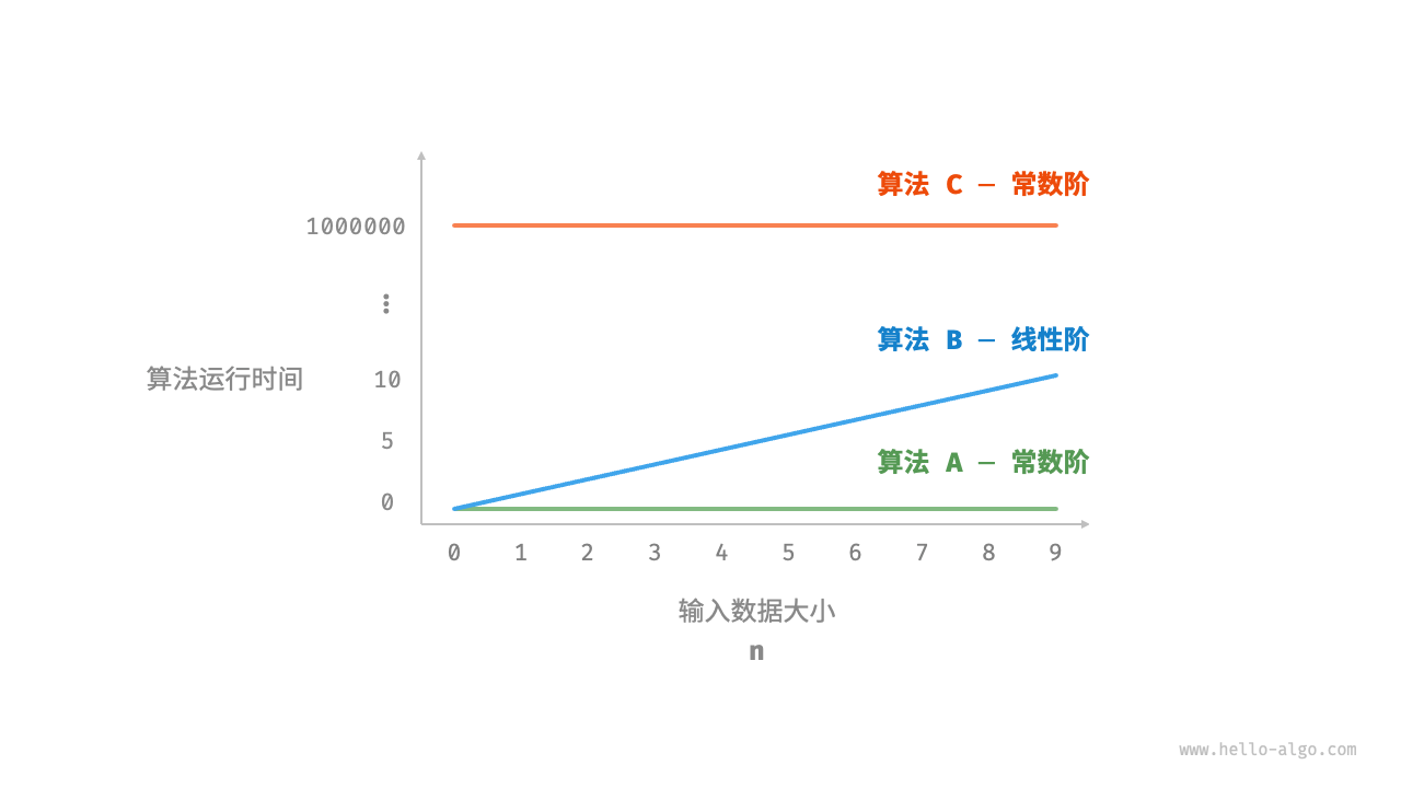
图 2-7   算法 A、B 和 C 的时间增长趋势

相较于直接统计算法的运行时间，时间复杂度分析有哪些特点呢？

• 时间复杂度能够有效评估算法效率。例如，算法 B 的运行时间呈线性增长，在 \(n > 1\) 时比算法 A 更慢，在 \(n > 1000000\) 时比算法 C 更慢。事实上，只要输入数据大小 \(n\) 足够大，复杂度为“常数阶”的算法一定优于“线性阶”的算法，这正是时间增长趋势的含义。
• 时间复杂度的推算方法更简便。显然，运行平台和计算操作类型都与算法运行时间的增长趋势无关。因此在时间复杂度分析中，我们可以简单地将所有计算操作的执行时间视为相同的“单位时间”，从而将“计算操作运行时间统计”简化为“计算操作数量统计”，这样一来估算难度就大大降低了。
• 时间复杂度也存在一定的局限性。例如，尽管算法 A 和 C 的时间复杂度相同，但实际运行时间差别很大。同样，尽管算法 B 的时间复杂度比 C 高，但在输入数据大小 \(n\) 较小时，算法 B 明显优于算法 C 。在这些情况下，我们很难仅凭时间复杂度判断算法效率的高低。当然，尽管存在上述问题，复杂度分析仍然是评判算法效率最有效且常用的方法。

2.3.2   函数渐近上界

给定一个输入大小为 \(n\) 的函数：

PythonC++JavaC#GoSwiftJSTSDartRustCKotlinRubyZig

def algorithm(n: int):
    a = 1      # +1
    a = a + 1  # +1
    a = a * 2  # +1
    # 循环 n 次
    for i in range(n):  # +1
        print(0)        # +1

void algorithm(int n) {
    int a = 1;  // +1
    a = a + 1;  // +1
    a = a * 2;  // +1
    // 循环 n 次
    for (int i = 0; i < n; i++) { // +1（每轮都执行 i ++）
        cout << 0 << endl;    // +1
    }
}

void algorithm(int n) {
    int a = 1;  // +1
    a = a + 1;  // +1
    a = a * 2;  // +1
    // 循环 n 次
    for (int i = 0; i < n; i++) { // +1（每轮都执行 i ++）
        System.out.println(0);    // +1
    }
}

void Algorithm(int n) {
    int a = 1;  // +1
    a = a + 1;  // +1
    a = a * 2;  // +1
    // 循环 n 次
    for (int i = 0; i < n; i++) {   // +1（每轮都执行 i ++）
        Console.WriteLine(0);   // +1
    }
}

func algorithm(n int) {
    a := 1      // +1
    a = a + 1   // +1
    a = a * 2   // +1
    // 循环 n 次
    for i := 0; i < n; i++ {   // +1
        fmt.Println(a)         // +1
    }
}

func algorithm(n: Int) {
    var a = 1 // +1
    a = a + 1 // +1
    a = a * 2 // +1
    // 循环 n 次
    for _ in 0 ..< n { // +1
        print(0) // +1
    }
}

function algorithm(n) {
    var a = 1; // +1
    a += 1; // +1
    a *= 2; // +1
    // 循环 n 次
    for(let i = 0; i < n; i++){ // +1（每轮都执行 i ++）
        console.log(0); // +1
    }
}

function algorithm(n: number): void{
    var a: number = 1; // +1
    a += 1; // +1
    a *= 2; // +1
    // 循环 n 次
    for(let i = 0; i < n; i++){ // +1（每轮都执行 i ++）
        console.log(0); // +1
    }
}

void algorithm(int n) {
  int a = 1; // +1
  a = a + 1; // +1
  a = a * 2; // +1
  // 循环 n 次
  for (int i = 0; i < n; i++) { // +1（每轮都执行 i ++）
    print(0); // +1
  }
}

fn algorithm(n: i32) {
    let mut a = 1;   // +1
    a = a + 1;      // +1
    a = a * 2;      // +1

    // 循环 n 次
    for _ in 0..n { // +1（每轮都执行 i ++）
        println!("{}", 0); // +1
    }
}

void algorithm(int n) {
    int a = 1;  // +1
    a = a + 1;  // +1
    a = a * 2;  // +1
    // 循环 n 次
    for (int i = 0; i < n; i++) {   // +1（每轮都执行 i ++）
        printf("%d", 0);            // +1
    }
}

fun algorithm(n: Int) {
    var a = 1 // +1
    a = a + 1 // +1
    a = a * 2 // +1
    // 循环 n 次
    for (i in 0..<n) { // +1（每轮都执行 i ++）
        println(0) // +1
    }
}

def algorithm(n)
    a = 1       # +1
    a = a + 1   # +1
    a = a * 2   # +1
    # 循环 n 次
    (0...n).each do # +1
        puts 0      # +1
    end
end

fn algorithm(n: usize) void {
    var a: i32 = 1; // +1
    a += 1; // +1
    a *= 2; // +1
    // 循环 n 次
    for (0..n) |_| { // +1（每轮都执行 i ++）
        std.debug.print("{}\n", .{0}); // +1
    }
}

设算法的操作数量是一个关于输入数据大小 \(n\) 的函数，记为 \(T(n)\) ，则以上函数的操作数量为：

\[ T(n) = 3 + 2n \]

\(T(n)\) 是一次函数，说明其运行时间的增长趋势是线性的，因此它的时间复杂度是线性阶。

我们将线性阶的时间复杂度记为 \(O(n)\) ，这个数学符号称为大 \(O\) 记号（big-\(O\) notation），表示函数 \(T(n)\) 的渐近上界（asymptotic upper bound）。

时间复杂度分析本质上是计算“操作数量 \(T(n)\)”的渐近上界，它具有明确的数学定义。

函数渐近上界

若存在正实数 \(c\) 和实数 \(n_0\) ，使得对于所有的 \(n > n_0\) ，均有 \(T(n) \leq c \cdot f(n)\) ，则可认为 \(f(n)\) 给出了 \(T(n)\) 的一个渐近上界，记为 \(T(n) = O(f(n))\) 。

如图 2-8 所示，计算渐近上界就是寻找一个函数 \(f(n)\) ，使得当 \(n\) 趋向于无穷大时，\(T(n)\) 和 \(f(n)\) 处于相同的增长级别，仅相差一个常数项 \(c\) 的倍数。

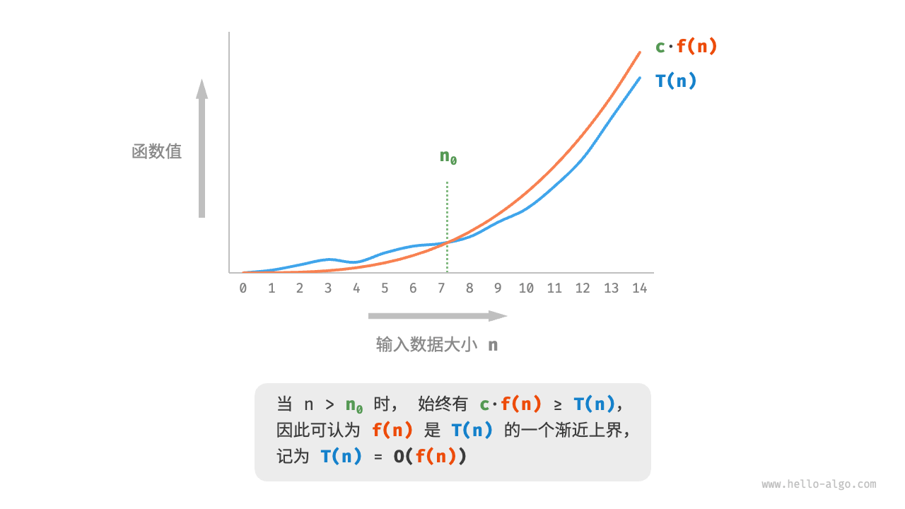
图 2-8   函数的渐近上界

2.3.3   推算方法

渐近上界的数学味儿有点重，如果你感觉没有完全理解，也无须担心。我们可以先掌握推算方法，在不断的实践中，就可以逐渐领悟其数学意义。

根据定义，确定 \(f(n)\) 之后，我们便可得到时间复杂度 \(O(f(n))\) 。那么如何确定渐近上界 \(f(n)\) 呢？总体分为两步：首先统计操作数量，然后判断渐近上界。

1.   第一步：统计操作数量

针对代码，逐行从上到下计算即可。然而，由于上述 \(c \cdot f(n)\) 中的常数项 \(c\) 可以取任意大小，因此操作数量 \(T(n)\) 中的各种系数、常数项都可以忽略。根据此原则，可以总结出以下计数简化技巧。

1. 忽略 \(T(n)\) 中的常数项。因为它们都与 \(n\) 无关，所以对时间复杂度不产生影响。
2. 省略所有系数。例如，循环 \(2n\) 次、\(5n + 1\) 次等，都可以简化记为 \(n\) 次，因为 \(n\) 前面的系数对时间复杂度没有影响。
3. 循环嵌套时使用乘法。总操作数量等于外层循环和内层循环操作数量之积，每一层循环依然可以分别套用第 1. 点和第 2. 点的技巧。

给定一个函数，我们可以用上述技巧来统计操作数量：

PythonC++JavaC#GoSwiftJSTSDartRustCKotlinRubyZig

def algorithm(n: int):
    a = 1      # +0（技巧 1）
    a = a + n  # +0（技巧 1）
    # +n（技巧 2）
    for i in range(5 * n + 1):
        print(0)
    # +n*n（技巧 3）
    for i in range(2 * n):
        for j in range(n + 1):
            print(0)

void algorithm(int n) {
    int a = 1;  // +0（技巧 1）
    a = a + n;  // +0（技巧 1）
    // +n（技巧 2）
    for (int i = 0; i < 5 * n + 1; i++) {
        cout << 0 << endl;
    }
    // +n*n（技巧 3）
    for (int i = 0; i < 2 * n; i++) {
        for (int j = 0; j < n + 1; j++) {
            cout << 0 << endl;
        }
    }
}

void algorithm(int n) {
    int a = 1;  // +0（技巧 1）
    a = a + n;  // +0（技巧 1）
    // +n（技巧 2）
    for (int i = 0; i < 5 * n + 1; i++) {
        System.out.println(0);
    }
    // +n*n（技巧 3）
    for (int i = 0; i < 2 * n; i++) {
        for (int j = 0; j < n + 1; j++) {
            System.out.println(0);
        }
    }
}

void Algorithm(int n) {
    int a = 1;  // +0（技巧 1）
    a = a + n;  // +0（技巧 1）
    // +n（技巧 2）
    for (int i = 0; i < 5 * n + 1; i++) {
        Console.WriteLine(0);
    }
    // +n*n（技巧 3）
    for (int i = 0; i < 2 * n; i++) {
        for (int j = 0; j < n + 1; j++) {
            Console.WriteLine(0);
        }
    }
}

func algorithm(n int) {
    a := 1     // +0（技巧 1）
    a = a + n  // +0（技巧 1）
    // +n（技巧 2）
    for i := 0; i < 5 * n + 1; i++ {
        fmt.Println(0)
    }
    // +n*n（技巧 3）
    for i := 0; i < 2 * n; i++ {
        for j := 0; j < n + 1; j++ {
            fmt.Println(0)
        }
    }
}

func algorithm(n: Int) {
    var a = 1 // +0（技巧 1）
    a = a + n // +0（技巧 1）
    // +n（技巧 2）
    for _ in 0 ..< (5 * n + 1) {
        print(0)
    }
    // +n*n（技巧 3）
    for _ in 0 ..< (2 * n) {
        for _ in 0 ..< (n + 1) {
            print(0)
        }
    }
}

function algorithm(n) {
    let a = 1;  // +0（技巧 1）
    a = a + n;  // +0（技巧 1）
    // +n（技巧 2）
    for (let i = 0; i < 5 * n + 1; i++) {
        console.log(0);
    }
    // +n*n（技巧 3）
    for (let i = 0; i < 2 * n; i++) {
        for (let j = 0; j < n + 1; j++) {
            console.log(0);
        }
    }
}

function algorithm(n: number): void {
    let a = 1;  // +0（技巧 1）
    a = a + n;  // +0（技巧 1）
    // +n（技巧 2）
    for (let i = 0; i < 5 * n + 1; i++) {
        console.log(0);
    }
    // +n*n（技巧 3）
    for (let i = 0; i < 2 * n; i++) {
        for (let j = 0; j < n + 1; j++) {
            console.log(0);
        }
    }
}

void algorithm(int n) {
  int a = 1; // +0（技巧 1）
  a = a + n; // +0（技巧 1）
  // +n（技巧 2）
  for (int i = 0; i < 5 * n + 1; i++) {
    print(0);
  }
  // +n*n（技巧 3）
  for (int i = 0; i < 2 * n; i++) {
    for (int j = 0; j < n + 1; j++) {
      print(0);
    }
  }
}

fn algorithm(n: i32) {
    let mut a = 1;     // +0（技巧 1）
    a = a + n;        // +0（技巧 1）

    // +n（技巧 2）
    for i in 0..(5 * n + 1) {
        println!("{}", 0);
    }

    // +n*n（技巧 3）
    for i in 0..(2 * n) {
        for j in 0..(n + 1) {
            println!("{}", 0);
        }
    }
}

void algorithm(int n) {
    int a = 1;  // +0（技巧 1）
    a = a + n;  // +0（技巧 1）
    // +n（技巧 2）
    for (int i = 0; i < 5 * n + 1; i++) {
        printf("%d", 0);
    }
    // +n*n（技巧 3）
    for (int i = 0; i < 2 * n; i++) {
        for (int j = 0; j < n + 1; j++) {
            printf("%d", 0);
        }
    }
}

fun algorithm(n: Int) {
    var a = 1   // +0（技巧 1）
    a = a + n   // +0（技巧 1）
    // +n（技巧 2）
    for (i in 0..<5 * n + 1) {
        println(0)
    }
    // +n*n（技巧 3）
    for (i in 0..<2 * n) {
        for (j in 0..<n + 1) {
            println(0)
        }
    }
}

def algorithm(n)
    a = 1       # +0（技巧 1）
    a = a + n   # +0（技巧 1）
    # +n（技巧 2）
    (0...(5 * n + 1)).each do { puts 0 }
    # +n*n（技巧 3）
    (0...(2 * n)).each do
        (0...(n + 1)).each do { puts 0 }
    end
end

fn algorithm(n: usize) void {
    var a: i32 = 1;     // +0（技巧 1）
    a = a + @as(i32, @intCast(n));        // +0（技巧 1）

    // +n（技巧 2）
    for(0..(5 * n + 1)) |_| {
        std.debug.print("{}\n", .{0});
    }

    // +n*n（技巧 3）
    for(0..(2 * n)) |_| {
        for(0..(n + 1)) |_| {
            std.debug.print("{}\n", .{0});
        }
    }
}

以下公式展示了使用上述技巧前后的统计结果，两者推算出的时间复杂度都为 \(O(n^2)\) 。

\[ \begin{aligned} T(n) & = 2n(n + 1) + (5n + 1) + 2 & \text{完整统计 (-.-|||)} \newline & = 2n^2 + 7n + 3 \newline T(n) & = n^2 + n & \text{偷懒统计 (o.O)} \end{aligned} \]

2.   第二步：判断渐近上界

时间复杂度由 \(T(n)\) 中最高阶的项来决定。这是因为在 \(n\) 趋于无穷大时，最高阶的项将发挥主导作用，其他项的影响都可以忽略。

表 2-2 展示了一些例子，其中一些夸张的值是为了强调“系数无法撼动阶数”这一结论。当 \(n\) 趋于无穷大时，这些常数变得无足轻重。

表 2-2   不同操作数量对应的时间复杂度

操作数量 \(T(n)\)	时间复杂度 \(O(f(n))\)
\(100000\)	\(O(1)\)
\(3n + 2\)	\(O(n)\)
\(2n^2 + 3n + 2\)	\(O(n^2)\)
\(n^3 + 10000n^2\)	\(O(n^3)\)
\(2^n + 10000n^{10000}\)	\(O(2^n)\)

2.3.4   常见类型

设输入数据大小为 \(n\) ，常见的时间复杂度类型如图 2-9 所示（按照从低到高的顺序排列）。

\[ \begin{aligned} O(1) < O(\log n) < O(n) < O(n \log n) < O(n^2) < O(2^n) < O(n!) \newline \text{常数阶} < \text{对数阶} < \text{线性阶} < \text{线性对数阶} < \text{平方阶} < \text{指数阶} < \text{阶乘阶} \end{aligned} \]

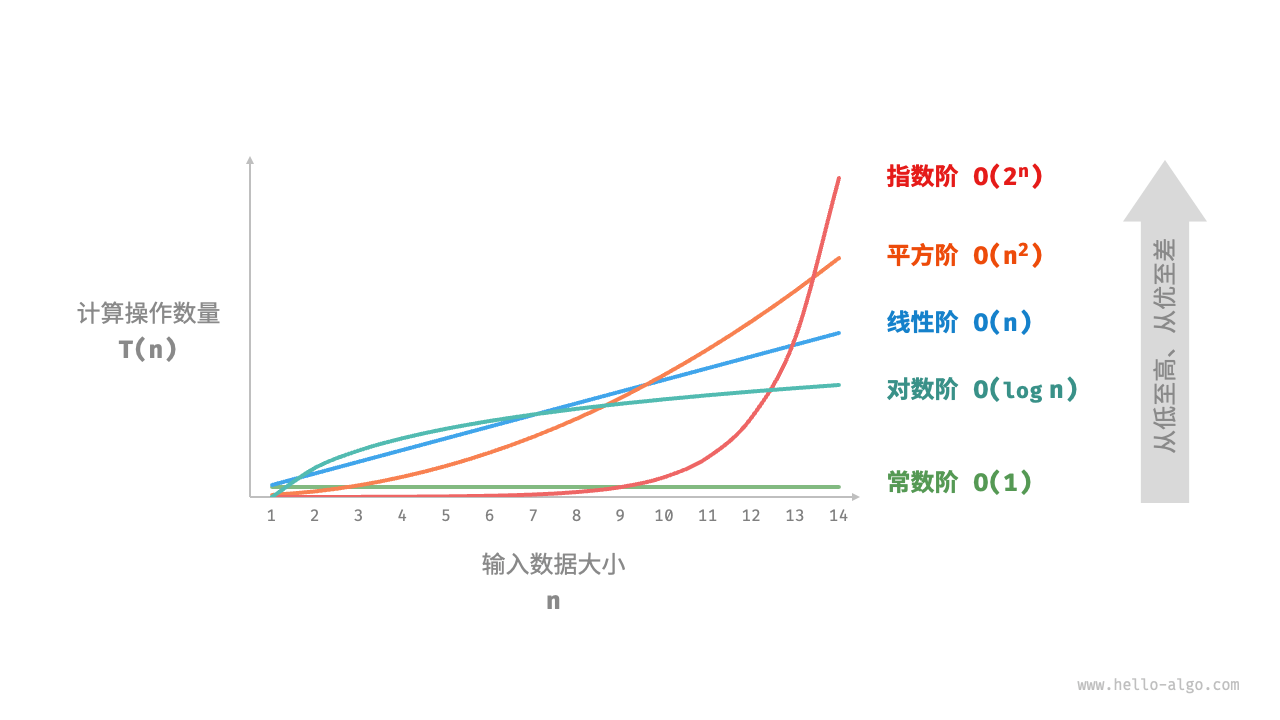
图 2-9   常见的时间复杂度类型

1.   常数阶 \(O(1)\)

常数阶的操作数量与输入数据大小 \(n\) 无关，即不随着 \(n\) 的变化而变化。

在以下函数中，尽管操作数量 size 可能很大，但由于其与输入数据大小 \(n\) 无关，因此时间复杂度仍为 \(O(1)\) ：

PythonC++JavaC#GoSwiftJSTSDartRustCKotlinRubyZig

time_complexity.py

def constant(n: int) -> int:
    """常数阶"""
    count = 0
    size = 100000
    for _ in range(size):
        count += 1
    return count

time_complexity.cpp

/* 常数阶 */
int constant(int n) {
    int count = 0;
    int size = 100000;
    for (int i = 0; i < size; i++)
        count++;
    return count;
}

time_complexity.java

/* 常数阶 */
int constant(int n) {
    int count = 0;
    int size = 100000;
    for (int i = 0; i < size; i++)
        count++;
    return count;
}

time_complexity.cs

/* 常数阶 */
int Constant(int n) {
    int count = 0;
    int size = 100000;
    for (int i = 0; i < size; i++)
        count++;
    return count;
}

time_complexity.go

/* 常数阶 */
func constant(n int) int {
    count := 0
    size := 100000
    for i := 0; i < size; i++ {
        count++
    }
    return count
}

time_complexity.swift

/* 常数阶 */
func constant(n: Int) -> Int {
    var count = 0
    let size = 100_000
    for _ in 0 ..< size {
        count += 1
    }
    return count
}

time_complexity.js

/* 常数阶 */
function constant(n) {
    let count = 0;
    const size = 100000;
    for (let i = 0; i < size; i++) count++;
    return count;
}

time_complexity.ts

/* 常数阶 */
function constant(n: number): number {
    let count = 0;
    const size = 100000;
    for (let i = 0; i < size; i++) count++;
    return count;
}

time_complexity.dart

/* 常数阶 */
int constant(int n) {
  int count = 0;
  int size = 100000;
  for (var i = 0; i < size; i++) {
    count++;
  }
  return count;
}

time_complexity.rs

/* 常数阶 */
fn constant(n: i32) -> i32 {
    _ = n;
    let mut count = 0;
    let size = 100_000;
    for _ in 0..size {
        count += 1;
    }
    count
}

time_complexity.c

/* 常数阶 */
int constant(int n) {
    int count = 0;
    int size = 100000;
    int i = 0;
    for (int i = 0; i < size; i++) {
        count++;
    }
    return count;
}

time_complexity.kt

/* 常数阶 */
fun constant(n: Int): Int {
    var count = 0
    val size = 100000
    for (i in 0..<size)
        count++
    return count
}

time_complexity.rb

### 常数阶 ###
def constant(n)
  count = 0
  size = 100000

  (0...size).each { count += 1 }

  count
end

time_complexity.zig

// 常数阶
fn constant(n: i32) i32 {
    _ = n;
    var count: i32 = 0;
    const size: i32 = 100_000;
    var i: i32 = 0;
    while(i<size) : (i += 1) {
        count += 1;
    }
    return count;
}

可视化运行

全屏观看 >

2.   线性阶 \(O(n)\)

线性阶的操作数量相对于输入数据大小 \(n\) 以线性级别增长。线性阶通常出现在单层循环中：

PythonC++JavaC#GoSwiftJSTSDartRustCKotlinRubyZig

time_complexity.py

def linear(n: int) -> int:
    """线性阶"""
    count = 0
    for _ in range(n):
        count += 1
    return count

time_complexity.cpp

/* 线性阶 */
int linear(int n) {
    int count = 0;
    for (int i = 0; i < n; i++)
        count++;
    return count;
}

time_complexity.java

/* 线性阶 */
int linear(int n) {
    int count = 0;
    for (int i = 0; i < n; i++)
        count++;
    return count;
}

time_complexity.cs

/* 线性阶 */
int Linear(int n) {
    int count = 0;
    for (int i = 0; i < n; i++)
        count++;
    return count;
}

time_complexity.go

/* 线性阶 */
func linear(n int) int {
    count := 0
    for i := 0; i < n; i++ {
        count++
    }
    return count
}

time_complexity.swift

/* 线性阶 */
func linear(n: Int) -> Int {
    var count = 0
    for _ in 0 ..< n {
        count += 1
    }
    return count
}

time_complexity.js

/* 线性阶 */
function linear(n) {
    let count = 0;
    for (let i = 0; i < n; i++) count++;
    return count;
}

time_complexity.ts

/* 线性阶 */
function linear(n: number): number {
    let count = 0;
    for (let i = 0; i < n; i++) count++;
    return count;
}

time_complexity.dart

/* 线性阶 */
int linear(int n) {
  int count = 0;
  for (var i = 0; i < n; i++) {
    count++;
  }
  return count;
}

time_complexity.rs

/* 线性阶 */
fn linear(n: i32) -> i32 {
    let mut count = 0;
    for _ in 0..n {
        count += 1;
    }
    count
}

time_complexity.c

/* 线性阶 */
int linear(int n) {
    int count = 0;
    for (int i = 0; i < n; i++) {
        count++;
    }
    return count;
}

time_complexity.kt

/* 线性阶 */
fun linear(n: Int): Int {
    var count = 0
    for (i in 0..<n)
        count++
    return count
}

time_complexity.rb

### 线性阶 ###
def linear(n)
  count = 0
  (0...n).each { count += 1 }
  count
end

time_complexity.zig

// 线性阶
fn linear(n: i32) i32 {
    var count: i32 = 0;
    var i: i32 = 0;
    while (i < n) : (i += 1) {
        count += 1;
    }
    return count;
}

可视化运行

全屏观看 >

遍历数组和遍历链表等操作的时间复杂度均为 \(O(n)\) ，其中 \(n\) 为数组或链表的长度：

PythonC++JavaC#GoSwiftJSTSDartRustCKotlinRubyZig

time_complexity.py

def array_traversal(nums: list[int]) -> int:
    """线性阶（遍历数组）"""
    count = 0
    # 循环次数与数组长度成正比
    for num in nums:
        count += 1
    return count

time_complexity.cpp

/* 线性阶（遍历数组） */
int arrayTraversal(vector<int> &nums) {
    int count = 0;
    // 循环次数与数组长度成正比
    for (int num : nums) {
        count++;
    }
    return count;
}

time_complexity.java

/* 线性阶（遍历数组） */
int arrayTraversal(int[] nums) {
    int count = 0;
    // 循环次数与数组长度成正比
    for (int num : nums) {
        count++;
    }
    return count;
}

time_complexity.cs

/* 线性阶（遍历数组） */
int ArrayTraversal(int[] nums) {
    int count = 0;
    // 循环次数与数组长度成正比
    foreach (int num in nums) {
        count++;
    }
    return count;
}

time_complexity.go

/* 线性阶（遍历数组） */
func arrayTraversal(nums []int) int {
    count := 0
    // 循环次数与数组长度成正比
    for range nums {
        count++
    }
    return count
}

time_complexity.swift

/* 线性阶（遍历数组） */
func arrayTraversal(nums: [Int]) -> Int {
    var count = 0
    // 循环次数与数组长度成正比
    for _ in nums {
        count += 1
    }
    return count
}

time_complexity.js

/* 线性阶（遍历数组） */
function arrayTraversal(nums) {
    let count = 0;
    // 循环次数与数组长度成正比
    for (let i = 0; i < nums.length; i++) {
        count++;
    }
    return count;
}

time_complexity.ts

/* 线性阶（遍历数组） */
function arrayTraversal(nums: number[]): number {
    let count = 0;
    // 循环次数与数组长度成正比
    for (let i = 0; i < nums.length; i++) {
        count++;
    }
    return count;
}

time_complexity.dart

/* 线性阶（遍历数组） */
int arrayTraversal(List<int> nums) {
  int count = 0;
  // 循环次数与数组长度成正比
  for (var _num in nums) {
    count++;
  }
  return count;
}

time_complexity.rs

/* 线性阶（遍历数组） */
fn array_traversal(nums: &[i32]) -> i32 {
    let mut count = 0;
    // 循环次数与数组长度成正比
    for _ in nums {
        count += 1;
    }
    count
}

time_complexity.c

/* 线性阶（遍历数组） */
int arrayTraversal(int *nums, int n) {
    int count = 0;
    // 循环次数与数组长度成正比
    for (int i = 0; i < n; i++) {
        count++;
    }
    return count;
}

time_complexity.kt

/* 线性阶（遍历数组） */
fun arrayTraversal(nums: IntArray): Int {
    var count = 0
    // 循环次数与数组长度成正比
    for (num in nums) {
        count++
    }
    return count
}

time_complexity.rb

### 线性阶（遍历数组）###
def array_traversal(nums)
  count = 0

  # 循环次数与数组长度成正比
  for num in nums
    count += 1
  end

  count
end

time_complexity.zig

// 线性阶（遍历数组）
fn arrayTraversal(nums: []i32) i32 {
    var count: i32 = 0;
    // 循环次数与数组长度成正比
    for (nums) |_| {
        count += 1;
    }
    return count;
}

可视化运行

全屏观看 >

值得注意的是，输入数据大小 \(n\) 需根据输入数据的类型来具体确定。比如在第一个示例中，变量 \(n\) 为输入数据大小；在第二个示例中，数组长度 \(n\) 为数据大小。

3.   平方阶 \(O(n^2)\)

平方阶的操作数量相对于输入数据大小 \(n\) 以平方级别增长。平方阶通常出现在嵌套循环中，外层循环和内层循环的时间复杂度都为 \(O(n)\) ，因此总体的时间复杂度为 \(O(n^2)\) ：

PythonC++JavaC#GoSwiftJSTSDartRustCKotlinRubyZig

time_complexity.py

def quadratic(n: int) -> int:
    """平方阶"""
    count = 0
    # 循环次数与数据大小 n 成平方关系
    for i in range(n):
        for j in range(n):
            count += 1
    return count

time_complexity.cpp

/* 平方阶 */
int quadratic(int n) {
    int count = 0;
    // 循环次数与数据大小 n 成平方关系
    for (int i = 0; i < n; i++) {
        for (int j = 0; j < n; j++) {
            count++;
        }
    }
    return count;
}

time_complexity.java

/* 平方阶 */
int quadratic(int n) {
    int count = 0;
    // 循环次数与数据大小 n 成平方关系
    for (int i = 0; i < n; i++) {
        for (int j = 0; j < n; j++) {
            count++;
        }
    }
    return count;
}

time_complexity.cs

/* 平方阶 */
int Quadratic(int n) {
    int count = 0;
    // 循环次数与数据大小 n 成平方关系
    for (int i = 0; i < n; i++) {
        for (int j = 0; j < n; j++) {
            count++;
        }
    }
    return count;
}

time_complexity.go

/* 平方阶 */
func quadratic(n int) int {
    count := 0
    // 循环次数与数据大小 n 成平方关系
    for i := 0; i < n; i++ {
        for j := 0; j < n; j++ {
            count++
        }
    }
    return count
}

time_complexity.swift

/* 平方阶 */
func quadratic(n: Int) -> Int {
    var count = 0
    // 循环次数与数据大小 n 成平方关系
    for _ in 0 ..< n {
        for _ in 0 ..< n {
            count += 1
        }
    }
    return count
}

time_complexity.js

/* 平方阶 */
function quadratic(n) {
    let count = 0;
    // 循环次数与数据大小 n 成平方关系
    for (let i = 0; i < n; i++) {
        for (let j = 0; j < n; j++) {
            count++;
        }
    }
    return count;
}

time_complexity.ts

/* 平方阶 */
function quadratic(n: number): number {
    let count = 0;
    // 循环次数与数据大小 n 成平方关系
    for (let i = 0; i < n; i++) {
        for (let j = 0; j < n; j++) {
            count++;
        }
    }
    return count;
}

time_complexity.dart

/* 平方阶 */
int quadratic(int n) {
  int count = 0;
  // 循环次数与数据大小 n 成平方关系
  for (int i = 0; i < n; i++) {
    for (int j = 0; j < n; j++) {
      count++;
    }
  }
  return count;
}

time_complexity.rs

/* 平方阶 */
fn quadratic(n: i32) -> i32 {
    let mut count = 0;
    // 循环次数与数据大小 n 成平方关系
    for _ in 0..n {
        for _ in 0..n {
            count += 1;
        }
    }
    count
}

time_complexity.c

/* 平方阶 */
int quadratic(int n) {
    int count = 0;
    // 循环次数与数据大小 n 成平方关系
    for (int i = 0; i < n; i++) {
        for (int j = 0; j < n; j++) {
            count++;
        }
    }
    return count;
}

time_complexity.kt

/* 平方阶 */
fun quadratic(n: Int): Int {
    var count = 0
    // 循环次数与数据大小 n 成平方关系
    for (i in 0..<n) {
        for (j in 0..<n) {
            count++
        }
    }
    return count
}

time_complexity.rb

### 平方阶 ###
def quadratic(n)
  count = 0

  # 循环次数与数据大小 n 成平方关系
  for i in 0...n
    for j in 0...n
      count += 1
    end
  end

  count
end

time_complexity.zig

// 平方阶
fn quadratic(n: i32) i32 {
    var count: i32 = 0;
    var i: i32 = 0;
    // 循环次数与数据大小 n 成平方关系
    while (i < n) : (i += 1) {
        var j: i32 = 0;
        while (j < n) : (j += 1) {
            count += 1;
        }
    }
    return count;
}

可视化运行

全屏观看 >

图 2-10 对比了常数阶、线性阶和平方阶三种时间复杂度。

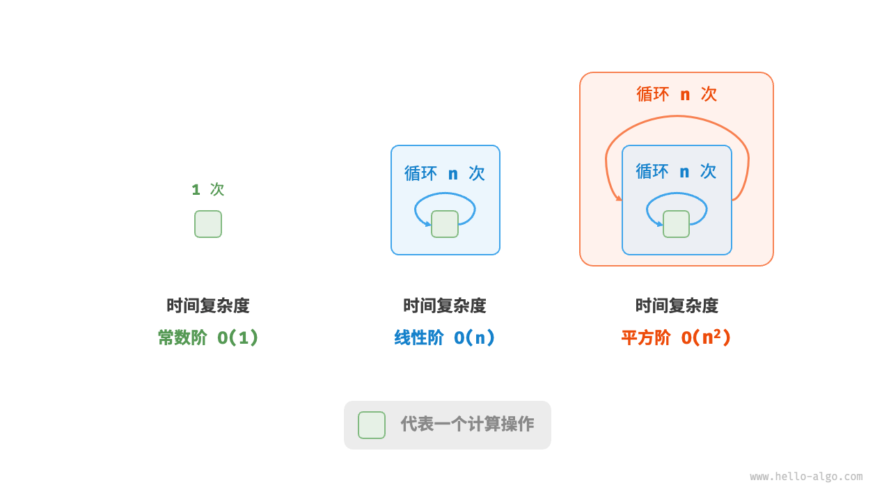
图 2-10   常数阶、线性阶和平方阶的时间复杂度

以冒泡排序为例，外层循环执行 \(n - 1\) 次，内层循环执行 \(n-1\)、\(n-2\)、\(\dots\)、\(2\)、\(1\) 次，平均为 \(n / 2\) 次，因此时间复杂度为 \(O((n - 1) n / 2) = O(n^2)\) ：

PythonC++JavaC#GoSwiftJSTSDartRustCKotlinRubyZig

time_complexity.py

def bubble_sort(nums: list[int]) -> int:
    """平方阶（冒泡排序）"""
    count = 0  # 计数器
    # 外循环：未排序区间为 [0, i]
    for i in range(len(nums) - 1, 0, -1):
        # 内循环：将未排序区间 [0, i] 中的最大元素交换至该区间的最右端
        for j in range(i):
            if nums[j] > nums[j + 1]:
                # 交换 nums[j] 与 nums[j + 1]
                tmp: int = nums[j]
                nums[j] = nums[j + 1]
                nums[j + 1] = tmp
                count += 3  # 元素交换包含 3 个单元操作
    return count

time_complexity.cpp

/* 平方阶（冒泡排序） */
int bubbleSort(vector<int> &nums) {
    int count = 0; // 计数器
    // 外循环：未排序区间为 [0, i]
    for (int i = nums.size() - 1; i > 0; i--) {
        // 内循环：将未排序区间 [0, i] 中的最大元素交换至该区间的最右端
        for (int j = 0; j < i; j++) {
            if (nums[j] > nums[j + 1]) {
                // 交换 nums[j] 与 nums[j + 1]
                int tmp = nums[j];
                nums[j] = nums[j + 1];
                nums[j + 1] = tmp;
                count += 3; // 元素交换包含 3 个单元操作
            }
        }
    }
    return count;
}

time_complexity.java

/* 平方阶（冒泡排序） */
int bubbleSort(int[] nums) {
    int count = 0; // 计数器
    // 外循环：未排序区间为 [0, i]
    for (int i = nums.length - 1; i > 0; i--) {
        // 内循环：将未排序区间 [0, i] 中的最大元素交换至该区间的最右端
        for (int j = 0; j < i; j++) {
            if (nums[j] > nums[j + 1]) {
                // 交换 nums[j] 与 nums[j + 1]
                int tmp = nums[j];
                nums[j] = nums[j + 1];
                nums[j + 1] = tmp;
                count += 3; // 元素交换包含 3 个单元操作
            }
        }
    }
    return count;
}

time_complexity.cs

/* 平方阶（冒泡排序） */
int BubbleSort(int[] nums) {
    int count = 0;  // 计数器
    // 外循环：未排序区间为 [0, i]
    for (int i = nums.Length - 1; i > 0; i--) {
        // 内循环：将未排序区间 [0, i] 中的最大元素交换至该区间的最右端
        for (int j = 0; j < i; j++) {
            if (nums[j] > nums[j + 1]) {
                // 交换 nums[j] 与 nums[j + 1]
                (nums[j + 1], nums[j]) = (nums[j], nums[j + 1]);
                count += 3;  // 元素交换包含 3 个单元操作
            }
        }
    }
    return count;
}

time_complexity.go

/* 平方阶（冒泡排序） */
func bubbleSort(nums []int) int {
    count := 0 // 计数器
    // 外循环：未排序区间为 [0, i]
    for i := len(nums) - 1; i > 0; i-- {
        // 内循环：将未排序区间 [0, i] 中的最大元素交换至该区间的最右端
        for j := 0; j < i; j++ {
            if nums[j] > nums[j+1] {
                // 交换 nums[j] 与 nums[j + 1]
                tmp := nums[j]
                nums[j] = nums[j+1]
                nums[j+1] = tmp
                count += 3 // 元素交换包含 3 个单元操作
            }
        }
    }
    return count
}

time_complexity.swift

/* 平方阶（冒泡排序） */
func bubbleSort(nums: inout [Int]) -> Int {
    var count = 0 // 计数器
    // 外循环：未排序区间为 [0, i]
    for i in nums.indices.dropFirst().reversed() {
        // 内循环：将未排序区间 [0, i] 中的最大元素交换至该区间的最右端
        for j in 0 ..< i {
            if nums[j] > nums[j + 1] {
                // 交换 nums[j] 与 nums[j + 1]
                let tmp = nums[j]
                nums[j] = nums[j + 1]
                nums[j + 1] = tmp
                count += 3 // 元素交换包含 3 个单元操作
            }
        }
    }
    return count
}

time_complexity.js

/* 平方阶（冒泡排序） */
function bubbleSort(nums) {
    let count = 0; // 计数器
    // 外循环：未排序区间为 [0, i]
    for (let i = nums.length - 1; i > 0; i--) {
        // 内循环：将未排序区间 [0, i] 中的最大元素交换至该区间的最右端
        for (let j = 0; j < i; j++) {
            if (nums[j] > nums[j + 1]) {
                // 交换 nums[j] 与 nums[j + 1]
                let tmp = nums[j];
                nums[j] = nums[j + 1];
                nums[j + 1] = tmp;
                count += 3; // 元素交换包含 3 个单元操作
            }
        }
    }
    return count;
}

time_complexity.ts

/* 平方阶（冒泡排序） */
function bubbleSort(nums: number[]): number {
    let count = 0; // 计数器
    // 外循环：未排序区间为 [0, i]
    for (let i = nums.length - 1; i > 0; i--) {
        // 内循环：将未排序区间 [0, i] 中的最大元素交换至该区间的最右端
        for (let j = 0; j < i; j++) {
            if (nums[j] > nums[j + 1]) {
                // 交换 nums[j] 与 nums[j + 1]
                let tmp = nums[j];
                nums[j] = nums[j + 1];
                nums[j + 1] = tmp;
                count += 3; // 元素交换包含 3 个单元操作
            }
        }
    }
    return count;
}

time_complexity.dart

/* 平方阶（冒泡排序） */
int bubbleSort(List<int> nums) {
  int count = 0; // 计数器
  // 外循环：未排序区间为 [0, i]
  for (var i = nums.length - 1; i > 0; i--) {
    // 内循环：将未排序区间 [0, i] 中的最大元素交换至该区间的最右端
    for (var j = 0; j < i; j++) {
      if (nums[j] > nums[j + 1]) {
        // 交换 nums[j] 与 nums[j + 1]
        int tmp = nums[j];
        nums[j] = nums[j + 1];
        nums[j + 1] = tmp;
        count += 3; // 元素交换包含 3 个单元操作
      }
    }
  }
  return count;
}

time_complexity.rs

/* 平方阶（冒泡排序） */
fn bubble_sort(nums: &mut [i32]) -> i32 {
    let mut count = 0; // 计数器

    // 外循环：未排序区间为 [0, i]
    for i in (1..nums.len()).rev() {
        // 内循环：将未排序区间 [0, i] 中的最大元素交换至该区间的最右端
        for j in 0..i {
            if nums[j] > nums[j + 1] {
                // 交换 nums[j] 与 nums[j + 1]
                let tmp = nums[j];
                nums[j] = nums[j + 1];
                nums[j + 1] = tmp;
                count += 3; // 元素交换包含 3 个单元操作
            }
        }
    }
    count
}

time_complexity.c

/* 平方阶（冒泡排序） */
int bubbleSort(int *nums, int n) {
    int count = 0; // 计数器
    // 外循环：未排序区间为 [0, i]
    for (int i = n - 1; i > 0; i--) {
        // 内循环：将未排序区间 [0, i] 中的最大元素交换至该区间的最右端
        for (int j = 0; j < i; j++) {
            if (nums[j] > nums[j + 1]) {
                // 交换 nums[j] 与 nums[j + 1]
                int tmp = nums[j];
                nums[j] = nums[j + 1];
                nums[j + 1] = tmp;
                count += 3; // 元素交换包含 3 个单元操作
            }
        }
    }
    return count;
}

time_complexity.kt

/* 平方阶（冒泡排序） */
fun bubbleSort(nums: IntArray): Int {
    var count = 0 // 计数器
    // 外循环：未排序区间为 [0, i]
    for (i in nums.size - 1 downTo 1) {
        // 内循环：将未排序区间 [0, i] 中的最大元素交换至该区间的最右端
        for (j in 0..<i) {
            if (nums[j] > nums[j + 1]) {
                // 交换 nums[j] 与 nums[j + 1]
                val temp = nums[j]
                nums[j] = nums[j + 1]
                nums[j + 1] = temp
                count += 3 // 元素交换包含 3 个单元操作
            }
        }
    }
    return count
}

time_complexity.rb

### 平方阶（冒泡排序）###
def bubble_sort(nums)
  count = 0  # 计数器

  # 外循环：未排序区间为 [0, i]
  for i in (nums.length - 1).downto(0)
    # 内循环：将未排序区间 [0, i] 中的最大元素交换至该区间的最右端
    for j in 0...i
      if nums[j] > nums[j + 1]
        # 交换 nums[j] 与 nums[j + 1]
        tmp = nums[j]
        nums[j] = nums[j + 1]
        nums[j + 1] = tmp
        count += 3 # 元素交换包含 3 个单元操作
      end
    end
  end

  count
end

time_complexity.zig

// 平方阶（冒泡排序）
fn bubbleSort(nums: []i32) i32 {
    var count: i32 = 0;  // 计数器 
    // 外循环：未排序区间为 [0, i]
    var i: i32 = @as(i32, @intCast(nums.len)) - 1;
    while (i > 0) : (i -= 1) {
        var j: usize = 0;
        // 内循环：将未排序区间 [0, i] 中的最大元素交换至该区间的最右端
        while (j < i) : (j += 1) {
            if (nums[j] > nums[j + 1]) {
                // 交换 nums[j] 与 nums[j + 1]
                var tmp = nums[j];
                nums[j] = nums[j + 1];
                nums[j + 1] = tmp;
                count += 3;  // 元素交换包含 3 个单元操作
            }
        }
    }
    return count;
}

可视化运行

全屏观看 >

4.   指数阶 \(O(2^n)\)

生物学的“细胞分裂”是指数阶增长的典型例子：初始状态为 \(1\) 个细胞，分裂一轮后变为 \(2\) 个，分裂两轮后变为 \(4\) 个，以此类推，分裂 \(n\) 轮后有 \(2^n\) 个细胞。

图 2-11 和以下代码模拟了细胞分裂的过程，时间复杂度为 \(O(2^n)\) ：

PythonC++JavaC#GoSwiftJSTSDartRustCKotlinRubyZig

time_complexity.py

def exponential(n: int) -> int:
    """指数阶（循环实现）"""
    count = 0
    base = 1
    # 细胞每轮一分为二，形成数列 1, 2, 4, 8, ..., 2^(n-1)
    for _ in range(n):
        for _ in range(base):
            count += 1
        base *= 2
    # count = 1 + 2 + 4 + 8 + .. + 2^(n-1) = 2^n - 1
    return count

time_complexity.cpp

/* 指数阶（循环实现） */
int exponential(int n) {
    int count = 0, base = 1;
    // 细胞每轮一分为二，形成数列 1, 2, 4, 8, ..., 2^(n-1)
    for (int i = 0; i < n; i++) {
        for (int j = 0; j < base; j++) {
            count++;
        }
        base *= 2;
    }
    // count = 1 + 2 + 4 + 8 + .. + 2^(n-1) = 2^n - 1
    return count;
}

time_complexity.java

/* 指数阶（循环实现） */
int exponential(int n) {
    int count = 0, base = 1;
    // 细胞每轮一分为二，形成数列 1, 2, 4, 8, ..., 2^(n-1)
    for (int i = 0; i < n; i++) {
        for (int j = 0; j < base; j++) {
            count++;
        }
        base *= 2;
    }
    // count = 1 + 2 + 4 + 8 + .. + 2^(n-1) = 2^n - 1
    return count;
}

time_complexity.cs

/* 指数阶（循环实现） */
int Exponential(int n) {
    int count = 0, bas = 1;
    // 细胞每轮一分为二，形成数列 1, 2, 4, 8, ..., 2^(n-1)
    for (int i = 0; i < n; i++) {
        for (int j = 0; j < bas; j++) {
            count++;
        }
        bas *= 2;
    }
    // count = 1 + 2 + 4 + 8 + .. + 2^(n-1) = 2^n - 1
    return count;
}

time_complexity.go

/* 指数阶（循环实现）*/
func exponential(n int) int {
    count, base := 0, 1
    // 细胞每轮一分为二，形成数列 1, 2, 4, 8, ..., 2^(n-1)
    for i := 0; i < n; i++ {
        for j := 0; j < base; j++ {
            count++
        }
        base *= 2
    }
    // count = 1 + 2 + 4 + 8 + .. + 2^(n-1) = 2^n - 1
    return count
}

time_complexity.swift

/* 指数阶（循环实现） */
func exponential(n: Int) -> Int {
    var count = 0
    var base = 1
    // 细胞每轮一分为二，形成数列 1, 2, 4, 8, ..., 2^(n-1)
    for _ in 0 ..< n {
        for _ in 0 ..< base {
            count += 1
        }
        base *= 2
    }
    // count = 1 + 2 + 4 + 8 + .. + 2^(n-1) = 2^n - 1
    return count
}

time_complexity.js

/* 指数阶（循环实现） */
function exponential(n) {
    let count = 0,
        base = 1;
    // 细胞每轮一分为二，形成数列 1, 2, 4, 8, ..., 2^(n-1)
    for (let i = 0; i < n; i++) {
        for (let j = 0; j < base; j++) {
            count++;
        }
        base *= 2;
    }
    // count = 1 + 2 + 4 + 8 + .. + 2^(n-1) = 2^n - 1
    return count;
}

time_complexity.ts

/* 指数阶（循环实现） */
function exponential(n: number): number {
    let count = 0,
        base = 1;
    // 细胞每轮一分为二，形成数列 1, 2, 4, 8, ..., 2^(n-1)
    for (let i = 0; i < n; i++) {
        for (let j = 0; j < base; j++) {
            count++;
        }
        base *= 2;
    }
    // count = 1 + 2 + 4 + 8 + .. + 2^(n-1) = 2^n - 1
    return count;
}

time_complexity.dart

/* 指数阶（循环实现） */
int exponential(int n) {
  int count = 0, base = 1;
  // 细胞每轮一分为二，形成数列 1, 2, 4, 8, ..., 2^(n-1)
  for (var i = 0; i < n; i++) {
    for (var j = 0; j < base; j++) {
      count++;
    }
    base *= 2;
  }
  // count = 1 + 2 + 4 + 8 + .. + 2^(n-1) = 2^n - 1
  return count;
}

time_complexity.rs

/* 指数阶（循环实现） */
fn exponential(n: i32) -> i32 {
    let mut count = 0;
    let mut base = 1;
    // 细胞每轮一分为二，形成数列 1, 2, 4, 8, ..., 2^(n-1)
    for _ in 0..n {
        for _ in 0..base {
            count += 1
        }
        base *= 2;
    }
    // count = 1 + 2 + 4 + 8 + .. + 2^(n-1) = 2^n - 1
    count
}

time_complexity.c

/* 指数阶（循环实现） */
int exponential(int n) {
    int count = 0;
    int bas = 1;
    // 细胞每轮一分为二，形成数列 1, 2, 4, 8, ..., 2^(n-1)
    for (int i = 0; i < n; i++) {
        for (int j = 0; j < bas; j++) {
            count++;
        }
        bas *= 2;
    }
    // count = 1 + 2 + 4 + 8 + .. + 2^(n-1) = 2^n - 1
    return count;
}

time_complexity.kt

/* 指数阶（循环实现） */
fun exponential(n: Int): Int {
    var count = 0
    var base = 1
    // 细胞每轮一分为二，形成数列 1, 2, 4, 8, ..., 2^(n-1)
    for (i in 0..<n) {
        for (j in 0..<base) {
            count++
        }
        base *= 2
    }
    // count = 1 + 2 + 4 + 8 + .. + 2^(n-1) = 2^n - 1
    return count
}

time_complexity.rb

### 指数阶（循环实现）###
def exponential(n)
  count, base = 0, 1

  # 细胞每轮一分为二，形成数列 1, 2, 4, 8, ..., 2^(n-1)
  (0...n).each do
    (0...base).each { count += 1 }
    base *= 2
  end

  # count = 1 + 2 + 4 + 8 + .. + 2^(n-1) = 2^n - 1
  count
end

time_complexity.zig

// 指数阶（循环实现）
fn exponential(n: i32) i32 {
    var count: i32 = 0;
    var bas: i32 = 1;
    var i: i32 = 0;
    // 细胞每轮一分为二，形成数列 1, 2, 4, 8, ..., 2^(n-1)
    while (i < n) : (i += 1) {
        var j: i32 = 0;
        while (j < bas) : (j += 1) {
            count += 1;
        }
        bas *= 2;
    }
    // count = 1 + 2 + 4 + 8 + .. + 2^(n-1) = 2^n - 1
    return count;
}

可视化运行

全屏观看 >

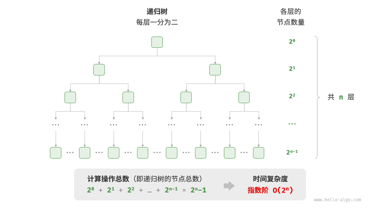
图 2-11   指数阶的时间复杂度

在实际算法中，指数阶常出现于递归函数中。例如在以下代码中，其递归地一分为二，经过 \(n\) 次分裂后停止：

PythonC++JavaC#GoSwiftJSTSDartRustCKotlinRubyZig

time_complexity.py

def exp_recur(n: int) -> int:
    """指数阶（递归实现）"""
    if n == 1:
        return 1
    return exp_recur(n - 1) + exp_recur(n - 1) + 1

time_complexity.cpp

/* 指数阶（递归实现） */
int expRecur(int n) {
    if (n == 1)
        return 1;
    return expRecur(n - 1) + expRecur(n - 1) + 1;
}

time_complexity.java

/* 指数阶（递归实现） */
int expRecur(int n) {
    if (n == 1)
        return 1;
    return expRecur(n - 1) + expRecur(n - 1) + 1;
}

time_complexity.cs

/* 指数阶（递归实现） */
int ExpRecur(int n) {
    if (n == 1) return 1;
    return ExpRecur(n - 1) + ExpRecur(n - 1) + 1;
}

time_complexity.go

/* 指数阶（递归实现）*/
func expRecur(n int) int {
    if n == 1 {
        return 1
    }
    return expRecur(n-1) + expRecur(n-1) + 1
}

time_complexity.swift

/* 指数阶（递归实现） */
func expRecur(n: Int) -> Int {
    if n == 1 {
        return 1
    }
    return expRecur(n: n - 1) + expRecur(n: n - 1) + 1
}

time_complexity.js

/* 指数阶（递归实现） */
function expRecur(n) {
    if (n === 1) return 1;
    return expRecur(n - 1) + expRecur(n - 1) + 1;
}

time_complexity.ts

/* 指数阶（递归实现） */
function expRecur(n: number): number {
    if (n === 1) return 1;
    return expRecur(n - 1) + expRecur(n - 1) + 1;
}

time_complexity.dart

/* 指数阶（递归实现） */
int expRecur(int n) {
  if (n == 1) return 1;
  return expRecur(n - 1) + expRecur(n - 1) + 1;
}

time_complexity.rs

/* 指数阶（递归实现） */
fn exp_recur(n: i32) -> i32 {
    if n == 1 {
        return 1;
    }
    exp_recur(n - 1) + exp_recur(n - 1) + 1
}

time_complexity.c

/* 指数阶（递归实现） */
int expRecur(int n) {
    if (n == 1)
        return 1;
    return expRecur(n - 1) + expRecur(n - 1) + 1;
}

time_complexity.kt

/* 指数阶（递归实现） */
fun expRecur(n: Int): Int {
    if (n == 1) {
        return 1
    }
    return expRecur(n - 1) + expRecur(n - 1) + 1
}

time_complexity.rb

### 指数阶（递归实现）###
def exp_recur(n)
  return 1 if n == 1
  exp_recur(n - 1) + exp_recur(n - 1) + 1
end

time_complexity.zig

// 指数阶（递归实现）
fn expRecur(n: i32) i32 {
    if (n == 1) return 1;
    return expRecur(n - 1) + expRecur(n - 1) + 1;
}

可视化运行

全屏观看 >

指数阶增长非常迅速，在穷举法（暴力搜索、回溯等）中比较常见。对于数据规模较大的问题，指数阶是不可接受的，通常需要使用动态规划或贪心算法等来解决。

5.   对数阶 \(O(\log n)\)

与指数阶相反，对数阶反映了“每轮缩减到一半”的情况。设输入数据大小为 \(n\) ，由于每轮缩减到一半，因此循环次数是 \(\log_2 n\) ，即 \(2^n\) 的反函数。

图 2-12 和以下代码模拟了“每轮缩减到一半”的过程，时间复杂度为 \(O(\log_2 n)\) ，简记为 \(O(\log n)\) ：

PythonC++JavaC#GoSwiftJSTSDartRustCKotlinRubyZig

time_complexity.py

def logarithmic(n: int) -> int:
    """对数阶（循环实现）"""
    count = 0
    while n > 1:
        n = n / 2
        count += 1
    return count

time_complexity.cpp

/* 对数阶（循环实现） */
int logarithmic(int n) {
    int count = 0;
    while (n > 1) {
        n = n / 2;
        count++;
    }
    return count;
}

time_complexity.java

/* 对数阶（循环实现） */
int logarithmic(int n) {
    int count = 0;
    while (n > 1) {
        n = n / 2;
        count++;
    }
    return count;
}

time_complexity.cs

/* 对数阶（循环实现） */
int Logarithmic(int n) {
    int count = 0;
    while (n > 1) {
        n /= 2;
        count++;
    }
    return count;
}

time_complexity.go

/* 对数阶（循环实现）*/
func logarithmic(n int) int {
    count := 0
    for n > 1 {
        n = n / 2
        count++
    }
    return count
}

time_complexity.swift

/* 对数阶（循环实现） */
func logarithmic(n: Int) -> Int {
    var count = 0
    var n = n
    while n > 1 {
        n = n / 2
        count += 1
    }
    return count
}

time_complexity.js

/* 对数阶（循环实现） */
function logarithmic(n) {
    let count = 0;
    while (n > 1) {
        n = n / 2;
        count++;
    }
    return count;
}

time_complexity.ts

/* 对数阶（循环实现） */
function logarithmic(n: number): number {
    let count = 0;
    while (n > 1) {
        n = n / 2;
        count++;
    }
    return count;
}

time_complexity.dart

/* 对数阶（循环实现） */
int logarithmic(int n) {
  int count = 0;
  while (n > 1) {
    n = n ~/ 2;
    count++;
  }
  return count;
}

time_complexity.rs

/* 对数阶（循环实现） */
fn logarithmic(mut n: i32) -> i32 {
    let mut count = 0;
    while n > 1 {
        n = n / 2;
        count += 1;
    }
    count
}

time_complexity.c

/* 对数阶（循环实现） */
int logarithmic(int n) {
    int count = 0;
    while (n > 1) {
        n = n / 2;
        count++;
    }
    return count;
}

time_complexity.kt

/* 对数阶（循环实现） */
fun logarithmic(n: Int): Int {
    var n1 = n
    var count = 0
    while (n1 > 1) {
        n1 /= 2
        count++
    }
    return count
}

time_complexity.rb

### 对数阶（循环实现）###
def logarithmic(n)
  count = 0

  while n > 1
    n /= 2
    count += 1
  end

  count
end

time_complexity.zig

// 对数阶（循环实现）
fn logarithmic(n: i32) i32 {
    var count: i32 = 0;
    var n_var = n;
    while (n_var > 1)
    {
        n_var = n_var / 2;
        count +=1;
    }
    return count;
}

可视化运行

全屏观看 >

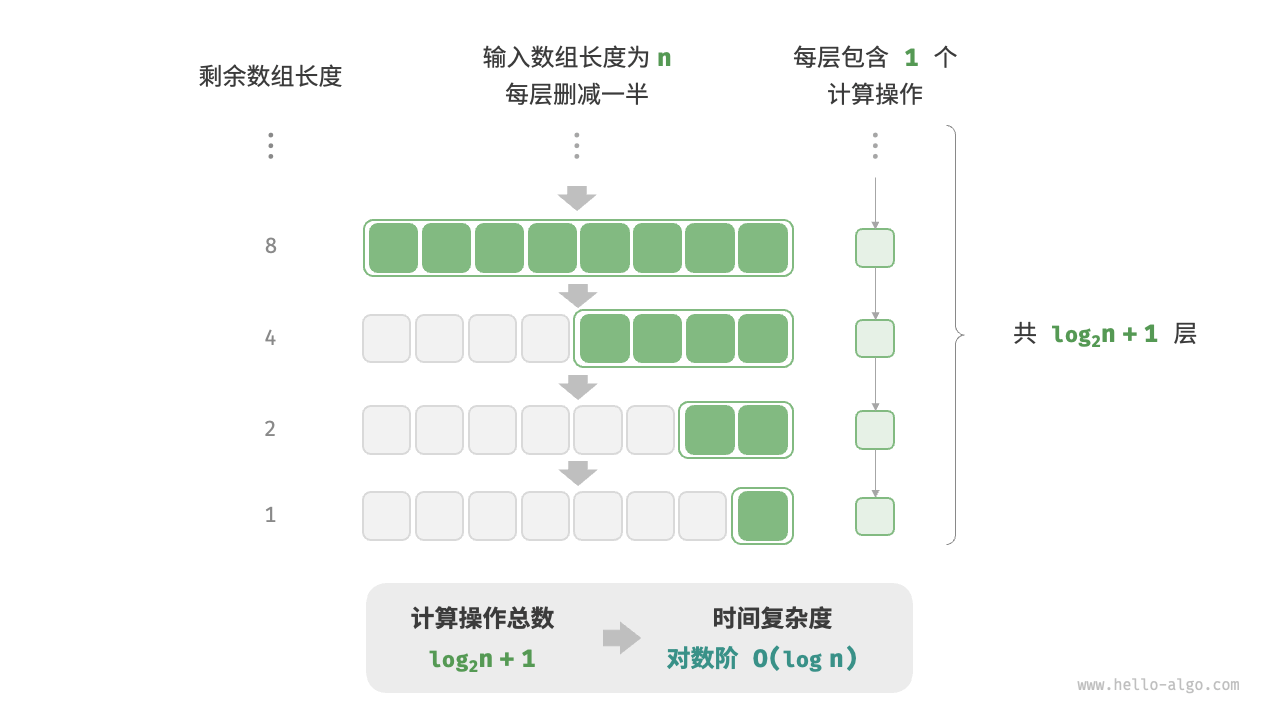
图 2-12   对数阶的时间复杂度

与指数阶类似，对数阶也常出现于递归函数中。以下代码形成了一棵高度为 \(\log_2 n\) 的递归树：

PythonC++JavaC#GoSwiftJSTSDartRustCKotlinRubyZig

time_complexity.py

def log_recur(n: int) -> int:
    """对数阶（递归实现）"""
    if n <= 1:
        return 0
    return log_recur(n / 2) + 1

time_complexity.cpp

/* 对数阶（递归实现） */
int logRecur(int n) {
    if (n <= 1)
        return 0;
    return logRecur(n / 2) + 1;
}

time_complexity.java

/* 对数阶（递归实现） */
int logRecur(int n) {
    if (n <= 1)
        return 0;
    return logRecur(n / 2) + 1;
}

time_complexity.cs

/* 对数阶（递归实现） */
int LogRecur(int n) {
    if (n <= 1) return 0;
    return LogRecur(n / 2) + 1;
}

time_complexity.go

/* 对数阶（递归实现）*/
func logRecur(n int) int {
    if n <= 1 {
        return 0
    }
    return logRecur(n/2) + 1
}

time_complexity.swift

/* 对数阶（递归实现） */
func logRecur(n: Int) -> Int {
    if n <= 1 {
        return 0
    }
    return logRecur(n: n / 2) + 1
}

time_complexity.js

/* 对数阶（递归实现） */
function logRecur(n) {
    if (n <= 1) return 0;
    return logRecur(n / 2) + 1;
}

time_complexity.ts

/* 对数阶（递归实现） */
function logRecur(n: number): number {
    if (n <= 1) return 0;
    return logRecur(n / 2) + 1;
}

time_complexity.dart

/* 对数阶（递归实现） */
int logRecur(int n) {
  if (n <= 1) return 0;
  return logRecur(n ~/ 2) + 1;
}

time_complexity.rs

/* 对数阶（递归实现） */
fn log_recur(n: i32) -> i32 {
    if n <= 1 {
        return 0;
    }
    log_recur(n / 2) + 1
}

time_complexity.c

/* 对数阶（递归实现） */
int logRecur(int n) {
    if (n <= 1)
        return 0;
    return logRecur(n / 2) + 1;
}

time_complexity.kt

/* 对数阶（递归实现） */
fun logRecur(n: Int): Int {
    if (n <= 1)
        return 0
    return logRecur(n / 2) + 1
}

time_complexity.rb

### 对数阶（递归实现）###
def log_recur(n)
  return 0 unless n > 1
  log_recur(n / 2) + 1
end

time_complexity.zig

// 对数阶（递归实现）
fn logRecur(n: i32) i32 {
    if (n <= 1) return 0;
    return logRecur(n / 2) + 1;
}

可视化运行

全屏观看 >

对数阶常出现于基于分治策略的算法中，体现了“一分为多”和“化繁为简”的算法思想。它增长缓慢，是仅次于常数阶的理想的时间复杂度。

\(O(\log n)\) 的底数是多少？

准确来说，“一分为 \(m\)”对应的时间复杂度是 \(O(\log_m n)\) 。而通过对数换底公式，我们可以得到具有不同底数、相等的时间复杂度：

\[ O(\log_m n) = O(\log_k n / \log_k m) = O(\log_k n) \]

也就是说，底数 \(m\) 可以在不影响复杂度的前提下转换。因此我们通常会省略底数 \(m\) ，将对数阶直接记为 \(O(\log n)\) 。

6.   线性对数阶 \(O(n \log n)\)

线性对数阶常出现于嵌套循环中，两层循环的时间复杂度分别为 \(O(\log n)\) 和 \(O(n)\) 。相关代码如下：

PythonC++JavaC#GoSwiftJSTSDartRustCKotlinRubyZig

time_complexity.py

def linear_log_recur(n: int) -> int:
    """线性对数阶"""
    if n <= 1:
        return 1
    count: int = linear_log_recur(n // 2) + linear_log_recur(n // 2)
    for _ in range(n):
        count += 1
    return count

time_complexity.cpp

/* 线性对数阶 */
int linearLogRecur(int n) {
    if (n <= 1)
        return 1;
    int count = linearLogRecur(n / 2) + linearLogRecur(n / 2);
    for (int i = 0; i < n; i++) {
        count++;
    }
    return count;
}

time_complexity.java

/* 线性对数阶 */
int linearLogRecur(int n) {
    if (n <= 1)
        return 1;
    int count = linearLogRecur(n / 2) + linearLogRecur(n / 2);
    for (int i = 0; i < n; i++) {
        count++;
    }
    return count;
}

time_complexity.cs

/* 线性对数阶 */
int LinearLogRecur(int n) {
    if (n <= 1) return 1;
    int count = LinearLogRecur(n / 2) + LinearLogRecur(n / 2);
    for (int i = 0; i < n; i++) {
        count++;
    }
    return count;
}

time_complexity.go

/* 线性对数阶 */
func linearLogRecur(n int) int {
    if n <= 1 {
        return 1
    }
    count := linearLogRecur(n/2) + linearLogRecur(n/2)
    for i := 0; i < n; i++ {
        count++
    }
    return count
}

time_complexity.swift

/* 线性对数阶 */
func linearLogRecur(n: Int) -> Int {
    if n <= 1 {
        return 1
    }
    var count = linearLogRecur(n: n / 2) + linearLogRecur(n: n / 2)
    for _ in stride(from: 0, to: n, by: 1) {
        count += 1
    }
    return count
}

time_complexity.js

/* 线性对数阶 */
function linearLogRecur(n) {
    if (n <= 1) return 1;
    let count = linearLogRecur(n / 2) + linearLogRecur(n / 2);
    for (let i = 0; i < n; i++) {
        count++;
    }
    return count;
}

time_complexity.ts

/* 线性对数阶 */
function linearLogRecur(n: number): number {
    if (n <= 1) return 1;
    let count = linearLogRecur(n / 2) + linearLogRecur(n / 2);
    for (let i = 0; i < n; i++) {
        count++;
    }
    return count;
}

time_complexity.dart

/* 线性对数阶 */
int linearLogRecur(int n) {
  if (n <= 1) return 1;
  int count = linearLogRecur(n ~/ 2) + linearLogRecur(n ~/ 2);
  for (var i = 0; i < n; i++) {
    count++;
  }
  return count;
}

time_complexity.rs

/* 线性对数阶 */
fn linear_log_recur(n: i32) -> i32 {
    if n <= 1 {
        return 1;
    }
    let mut count = linear_log_recur(n / 2) + linear_log_recur(n / 2);
    for _ in 0..n as i32 {
        count += 1;
    }
    return count;
}

time_complexity.c

/* 线性对数阶 */
int linearLogRecur(int n) {
    if (n <= 1)
        return 1;
    int count = linearLogRecur(n / 2) + linearLogRecur(n / 2);
    for (int i = 0; i < n; i++) {
        count++;
    }
    return count;
}

time_complexity.kt

/* 线性对数阶 */
fun linearLogRecur(n: Int): Int {
    if (n <= 1)
        return 1
    var count = linearLogRecur(n / 2) + linearLogRecur(n / 2)
    for (i in 0..<n) {
        count++
    }
    return count
}

time_complexity.rb

### 线性对数阶 ###
def linear_log_recur(n)
  return 1 unless n > 1

  count = linear_log_recur(n / 2) + linear_log_recur(n / 2)
  (0...n).each { count += 1 }

  count
end

time_complexity.zig

// 线性对数阶
fn linearLogRecur(n: i32) i32 {
    if (n <= 1) return 1;
    var count: i32 = linearLogRecur(n / 2) + linearLogRecur(n / 2);
    var i: i32 = 0;
    while (i < n) : (i += 1) {
        count += 1;
    }
    return count;
}

可视化运行

全屏观看 >

图 2-13 展示了线性对数阶的生成方式。二叉树的每一层的操作总数都为 \(n\) ，树共有 \(\log_2 n + 1\) 层，因此时间复杂度为 \(O(n \log n)\) 。

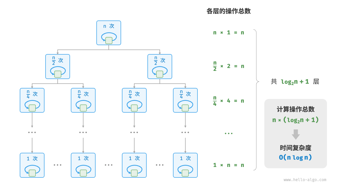
图 2-13   线性对数阶的时间复杂度

主流排序算法的时间复杂度通常为 \(O(n \log n)\) ，例如快速排序、归并排序、堆排序等。

7.   阶乘阶 \(O(n!)\)

阶乘阶对应数学上的“全排列”问题。给定 \(n\) 个互不重复的元素，求其所有可能的排列方案，方案数量为：

\[ n! = n \times (n - 1) \times (n - 2) \times \dots \times 2 \times 1 \]

阶乘通常使用递归实现。如图 2-14 和以下代码所示，第一层分裂出 \(n\) 个，第二层分裂出 \(n - 1\) 个，以此类推，直至第 \(n\) 层时停止分裂：

PythonC++JavaC#GoSwiftJSTSDartRustCKotlinRubyZig

time_complexity.py

def factorial_recur(n: int) -> int:
    """阶乘阶（递归实现）"""
    if n == 0:
        return 1
    count = 0
    # 从 1 个分裂出 n 个
    for _ in range(n):
        count += factorial_recur(n - 1)
    return count

time_complexity.cpp

/* 阶乘阶（递归实现） */
int factorialRecur(int n) {
    if (n == 0)
        return 1;
    int count = 0;
    // 从 1 个分裂出 n 个
    for (int i = 0; i < n; i++) {
        count += factorialRecur(n - 1);
    }
    return count;
}

time_complexity.java

/* 阶乘阶（递归实现） */
int factorialRecur(int n) {
    if (n == 0)
        return 1;
    int count = 0;
    // 从 1 个分裂出 n 个
    for (int i = 0; i < n; i++) {
        count += factorialRecur(n - 1);
    }
    return count;
}

time_complexity.cs

/* 阶乘阶（递归实现） */
int FactorialRecur(int n) {
    if (n == 0) return 1;
    int count = 0;
    // 从 1 个分裂出 n 个
    for (int i = 0; i < n; i++) {
        count += FactorialRecur(n - 1);
    }
    return count;
}

time_complexity.go

/* 阶乘阶（递归实现） */
func factorialRecur(n int) int {
    if n == 0 {
        return 1
    }
    count := 0
    // 从 1 个分裂出 n 个
    for i := 0; i < n; i++ {
        count += factorialRecur(n - 1)
    }
    return count
}

time_complexity.swift

/* 阶乘阶（递归实现） */
func factorialRecur(n: Int) -> Int {
    if n == 0 {
        return 1
    }
    var count = 0
    // 从 1 个分裂出 n 个
    for _ in 0 ..< n {
        count += factorialRecur(n: n - 1)
    }
    return count
}

time_complexity.js

/* 阶乘阶（递归实现） */
function factorialRecur(n) {
    if (n === 0) return 1;
    let count = 0;
    // 从 1 个分裂出 n 个
    for (let i = 0; i < n; i++) {
        count += factorialRecur(n - 1);
    }
    return count;
}

time_complexity.ts

/* 阶乘阶（递归实现） */
function factorialRecur(n: number): number {
    if (n === 0) return 1;
    let count = 0;
    // 从 1 个分裂出 n 个
    for (let i = 0; i < n; i++) {
        count += factorialRecur(n - 1);
    }
    return count;
}

time_complexity.dart

/* 阶乘阶（递归实现） */
int factorialRecur(int n) {
  if (n == 0) return 1;
  int count = 0;
  // 从 1 个分裂出 n 个
  for (var i = 0; i < n; i++) {
    count += factorialRecur(n - 1);
  }
  return count;
}

time_complexity.rs

/* 阶乘阶（递归实现） */
fn factorial_recur(n: i32) -> i32 {
    if n == 0 {
        return 1;
    }
    let mut count = 0;
    // 从 1 个分裂出 n 个
    for _ in 0..n {
        count += factorial_recur(n - 1);
    }
    count
}

time_complexity.c

/* 阶乘阶（递归实现） */
int factorialRecur(int n) {
    if (n == 0)
        return 1;
    int count = 0;
    for (int i = 0; i < n; i++) {
        count += factorialRecur(n - 1);
    }
    return count;
}

time_complexity.kt

/* 阶乘阶（递归实现） */
fun factorialRecur(n: Int): Int {
    if (n == 0)
        return 1
    var count = 0
    // 从 1 个分裂出 n 个
    for (i in 0..<n) {
        count += factorialRecur(n - 1)
    }
    return count
}

time_complexity.rb

### 阶乘阶（递归实现）###
def factorial_recur(n)
  return 1 if n == 0

  count = 0
  # 从 1 个分裂出 n 个
  (0...n).each { count += factorial_recur(n - 1) }

  count
end

time_complexity.zig

// 阶乘阶（递归实现）
fn factorialRecur(n: i32) i32 {
    if (n == 0) return 1;
    var count: i32 = 0;
    var i: i32 = 0;
    // 从 1 个分裂出 n 个
    while (i < n) : (i += 1) {
        count += factorialRecur(n - 1);
    }
    return count;
}

可视化运行

全屏观看 >

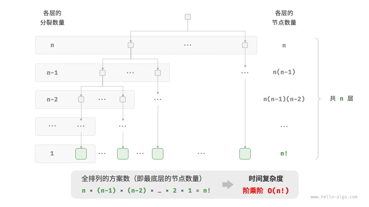
图 2-14   阶乘阶的时间复杂度

请注意，因为当 \(n \geq 4\) 时恒有 \(n! > 2^n\) ，所以阶乘阶比指数阶增长得更快，在 \(n\) 较大时也是不可接受的。

2.3.5   最差、最佳、平均时间复杂度

算法的时间效率往往不是固定的，而是与输入数据的分布有关。假设输入一个长度为 \(n\) 的数组 nums ，其中 nums 由从 \(1\) 至 \(n\) 的数字组成，每个数字只出现一次；但元素顺序是随机打乱的，任务目标是返回元素 \(1\) 的索引。我们可以得出以下结论。

• 当 nums = [?, ?, ..., 1] ，即当末尾元素是 \(1\) 时，需要完整遍历数组，达到最差时间复杂度 \(O(n)\) 。
• 当 nums = [1, ?, ?, ...] ，即当首个元素为 \(1\) 时，无论数组多长都不需要继续遍历，达到最佳时间复杂度 \(\Omega(1)\) 。

“最差时间复杂度”对应函数渐近上界，使用大 \(O\) 记号表示。相应地，“最佳时间复杂度”对应函数渐近下界，用 \(\Omega\) 记号表示：

PythonC++JavaC#GoSwiftJSTSDartRustCKotlinRubyZig

worst_best_time_complexity.py

def random_numbers(n: int) -> list[int]:
    """生成一个数组，元素为: 1, 2, ..., n ，顺序被打乱"""
    # 生成数组 nums =: 1, 2, 3, ..., n
    nums = [i for i in range(1, n + 1)]
    # 随机打乱数组元素
    random.shuffle(nums)
    return nums

def find_one(nums: list[int]) -> int:
    """查找数组 nums 中数字 1 所在索引"""
    for i in range(len(nums)):
        # 当元素 1 在数组头部时，达到最佳时间复杂度 O(1)
        # 当元素 1 在数组尾部时，达到最差时间复杂度 O(n)
        if nums[i] == 1:
            return i
    return -1

worst_best_time_complexity.cpp

/* 生成一个数组，元素为 { 1, 2, ..., n }，顺序被打乱 */
vector<int> randomNumbers(int n) {
    vector<int> nums(n);
    // 生成数组 nums = { 1, 2, 3, ..., n }
    for (int i = 0; i < n; i++) {
        nums[i] = i + 1;
    }
    // 使用系统时间生成随机种子
    unsigned seed = chrono::system_clock::now().time_since_epoch().count();
    // 随机打乱数组元素
    shuffle(nums.begin(), nums.end(), default_random_engine(seed));
    return nums;
}

/* 查找数组 nums 中数字 1 所在索引 */
int findOne(vector<int> &nums) {
    for (int i = 0; i < nums.size(); i++) {
        // 当元素 1 在数组头部时，达到最佳时间复杂度 O(1)
        // 当元素 1 在数组尾部时，达到最差时间复杂度 O(n)
        if (nums[i] == 1)
            return i;
    }
    return -1;
}

worst_best_time_complexity.java

/* 生成一个数组，元素为 { 1, 2, ..., n }，顺序被打乱 */
int[] randomNumbers(int n) {
    Integer[] nums = new Integer[n];
    // 生成数组 nums = { 1, 2, 3, ..., n }
    for (int i = 0; i < n; i++) {
        nums[i] = i + 1;
    }
    // 随机打乱数组元素
    Collections.shuffle(Arrays.asList(nums));
    // Integer[] -> int[]
    int[] res = new int[n];
    for (int i = 0; i < n; i++) {
        res[i] = nums[i];
    }
    return res;
}

/* 查找数组 nums 中数字 1 所在索引 */
int findOne(int[] nums) {
    for (int i = 0; i < nums.length; i++) {
        // 当元素 1 在数组头部时，达到最佳时间复杂度 O(1)
        // 当元素 1 在数组尾部时，达到最差时间复杂度 O(n)
        if (nums[i] == 1)
            return i;
    }
    return -1;
}

worst_best_time_complexity.cs

/* 生成一个数组，元素为 { 1, 2, ..., n }，顺序被打乱 */
int[] RandomNumbers(int n) {
    int[] nums = new int[n];
    // 生成数组 nums = { 1, 2, 3, ..., n }
    for (int i = 0; i < n; i++) {
        nums[i] = i + 1;
    }

    // 随机打乱数组元素
    for (int i = 0; i < nums.Length; i++) {
        int index = new Random().Next(i, nums.Length);
        (nums[i], nums[index]) = (nums[index], nums[i]);
    }
    return nums;
}

/* 查找数组 nums 中数字 1 所在索引 */
int FindOne(int[] nums) {
    for (int i = 0; i < nums.Length; i++) {
        // 当元素 1 在数组头部时，达到最佳时间复杂度 O(1)
        // 当元素 1 在数组尾部时，达到最差时间复杂度 O(n)
        if (nums[i] == 1)
            return i;
    }
    return -1;
}

worst_best_time_complexity.go

/* 生成一个数组，元素为 { 1, 2, ..., n }，顺序被打乱 */
func randomNumbers(n int) []int {
    nums := make([]int, n)
    // 生成数组 nums = { 1, 2, 3, ..., n }
    for i := 0; i < n; i++ {
        nums[i] = i + 1
    }
    // 随机打乱数组元素
    rand.Shuffle(len(nums), func(i, j int) {
        nums[i], nums[j] = nums[j], nums[i]
    })
    return nums
}

/* 查找数组 nums 中数字 1 所在索引 */
func findOne(nums []int) int {
    for i := 0; i < len(nums); i++ {
        // 当元素 1 在数组头部时，达到最佳时间复杂度 O(1)
        // 当元素 1 在数组尾部时，达到最差时间复杂度 O(n)
        if nums[i] == 1 {
            return i
        }
    }
    return -1
}

worst_best_time_complexity.swift

/* 生成一个数组，元素为 { 1, 2, ..., n }，顺序被打乱 */
func randomNumbers(n: Int) -> [Int] {
    // 生成数组 nums = { 1, 2, 3, ..., n }
    var nums = Array(1 ... n)
    // 随机打乱数组元素
    nums.shuffle()
    return nums
}

/* 查找数组 nums 中数字 1 所在索引 */
func findOne(nums: [Int]) -> Int {
    for i in nums.indices {
        // 当元素 1 在数组头部时，达到最佳时间复杂度 O(1)
        // 当元素 1 在数组尾部时，达到最差时间复杂度 O(n)
        if nums[i] == 1 {
            return i
        }
    }
    return -1
}

worst_best_time_complexity.js

/* 生成一个数组，元素为 { 1, 2, ..., n }，顺序被打乱 */
function randomNumbers(n) {
    const nums = Array(n);
    // 生成数组 nums = { 1, 2, 3, ..., n }
    for (let i = 0; i < n; i++) {
        nums[i] = i + 1;
    }
    // 随机打乱数组元素
    for (let i = 0; i < n; i++) {
        const r = Math.floor(Math.random() * (i + 1));
        const temp = nums[i];
        nums[i] = nums[r];
        nums[r] = temp;
    }
    return nums;
}

/* 查找数组 nums 中数字 1 所在索引 */
function findOne(nums) {
    for (let i = 0; i < nums.length; i++) {
        // 当元素 1 在数组头部时，达到最佳时间复杂度 O(1)
        // 当元素 1 在数组尾部时，达到最差时间复杂度 O(n)
        if (nums[i] === 1) {
            return i;
        }
    }
    return -1;
}

worst_best_time_complexity.ts

/* 生成一个数组，元素为 { 1, 2, ..., n }，顺序被打乱 */
function randomNumbers(n: number): number[] {
    const nums = Array(n);
    // 生成数组 nums = { 1, 2, 3, ..., n }
    for (let i = 0; i < n; i++) {
        nums[i] = i + 1;
    }
    // 随机打乱数组元素
    for (let i = 0; i < n; i++) {
        const r = Math.floor(Math.random() * (i + 1));
        const temp = nums[i];
        nums[i] = nums[r];
        nums[r] = temp;
    }
    return nums;
}

/* 查找数组 nums 中数字 1 所在索引 */
function findOne(nums: number[]): number {
    for (let i = 0; i < nums.length; i++) {
        // 当元素 1 在数组头部时，达到最佳时间复杂度 O(1)
        // 当元素 1 在数组尾部时，达到最差时间复杂度 O(n)
        if (nums[i] === 1) {
            return i;
        }
    }
    return -1;
}

worst_best_time_complexity.dart

/* 生成一个数组，元素为 { 1, 2, ..., n }，顺序被打乱 */
List<int> randomNumbers(int n) {
  final nums = List.filled(n, 0);
  // 生成数组 nums = { 1, 2, 3, ..., n }
  for (var i = 0; i < n; i++) {
    nums[i] = i + 1;
  }
  // 随机打乱数组元素
  nums.shuffle();

  return nums;
}

/* 查找数组 nums 中数字 1 所在索引 */
int findOne(List<int> nums) {
  for (var i = 0; i < nums.length; i++) {
    // 当元素 1 在数组头部时，达到最佳时间复杂度 O(1)
    // 当元素 1 在数组尾部时，达到最差时间复杂度 O(n)
    if (nums[i] == 1) return i;
  }

  return -1;
}

worst_best_time_complexity.rs

/* 生成一个数组，元素为 { 1, 2, ..., n }，顺序被打乱 */
fn random_numbers(n: i32) -> Vec<i32> {
    // 生成数组 nums = { 1, 2, 3, ..., n }
    let mut nums = (1..=n).collect::<Vec<i32>>();
    // 随机打乱数组元素
    nums.shuffle(&mut thread_rng());
    nums
}

/* 查找数组 nums 中数字 1 所在索引 */
fn find_one(nums: &[i32]) -> Option<usize> {
    for i in 0..nums.len() {
        // 当元素 1 在数组头部时，达到最佳时间复杂度 O(1)
        // 当元素 1 在数组尾部时，达到最差时间复杂度 O(n)
        if nums[i] == 1 {
            return Some(i);
        }
    }
    None
}

worst_best_time_complexity.c

/* 生成一个数组，元素为 { 1, 2, ..., n }，顺序被打乱 */
int *randomNumbers(int n) {
    // 分配堆区内存（创建一维可变长数组：数组中元素数量为 n ，元素类型为 int ）
    int *nums = (int *)malloc(n * sizeof(int));
    // 生成数组 nums = { 1, 2, 3, ..., n }
    for (int i = 0; i < n; i++) {
        nums[i] = i + 1;
    }
    // 随机打乱数组元素
    for (int i = n - 1; i > 0; i--) {
        int j = rand() % (i + 1);
        int temp = nums[i];
        nums[i] = nums[j];
        nums[j] = temp;
    }
    return nums;
}

/* 查找数组 nums 中数字 1 所在索引 */
int findOne(int *nums, int n) {
    for (int i = 0; i < n; i++) {
        // 当元素 1 在数组头部时，达到最佳时间复杂度 O(1)
        // 当元素 1 在数组尾部时，达到最差时间复杂度 O(n)
        if (nums[i] == 1)
            return i;
    }
    return -1;
}

worst_best_time_complexity.kt

/* 生成一个数组，元素为 { 1, 2, ..., n }，顺序被打乱 */
fun randomNumbers(n: Int): Array<Int?> {
    val nums = IntArray(n)
    // 生成数组 nums = { 1, 2, 3, ..., n }
    for (i in 0..<n) {
        nums[i] = i + 1
    }
    // 随机打乱数组元素
    nums.shuffle()
    val res = arrayOfNulls<Int>(n)
    for (i in 0..<n) {
        res[i] = nums[i]
    }
    return res
}

/* 查找数组 nums 中数字 1 所在索引 */
fun findOne(nums: Array<Int?>): Int {
    for (i in nums.indices) {
        // 当元素 1 在数组头部时，达到最佳时间复杂度 O(1)
        // 当元素 1 在数组尾部时，达到最差时间复杂度 O(n)
        if (nums[i] == 1)
            return i
    }
    return -1
}

worst_best_time_complexity.rb

### 生成一个数组，元素为: 1, 2, ..., n ，顺序被打乱 ###
def random_numbers(n)
  # 生成数组 nums =: 1, 2, 3, ..., n
  nums = Array.new(n) { |i| i + 1 }
  # 随机打乱数组元素
  nums.shuffle!
end

### 查找数组 nums 中数字 1 所在索引 ###
def find_one(nums)
  for i in 0...nums.length
    # 当元素 1 在数组头部时，达到最佳时间复杂度 O(1)
    # 当元素 1 在数组尾部时，达到最差时间复杂度 O(n)
    return i if nums[i] == 1
  end

  -1
end

worst_best_time_complexity.zig

// 生成一个数组，元素为 { 1, 2, ..., n }，顺序被打乱
fn randomNumbers(comptime n: usize) [n]i32 {
    var nums: [n]i32 = undefined;
    // 生成数组 nums = { 1, 2, 3, ..., n }
    for (&nums, 0..) |*num, i| {
        num.* = @as(i32, @intCast(i)) + 1;
    }
    // 随机打乱数组元素
    const rand = std.crypto.random;
    rand.shuffle(i32, &nums);
    return nums;
}

// 查找数组 nums 中数字 1 所在索引
fn findOne(nums: []i32) i32 {
    for (nums, 0..) |num, i| {
        // 当元素 1 在数组头部时，达到最佳时间复杂度 O(1)
        // 当元素 1 在数组尾部时，达到最差时间复杂度 O(n)
        if (num == 1) return @intCast(i);
    }
    return -1;
}

可视化运行

全屏观看 >

值得说明的是，我们在实际中很少使用最佳时间复杂度，因为通常只有在很小概率下才能达到，可能会带来一定的误导性。而最差时间复杂度更为实用，因为它给出了一个效率安全值，让我们可以放心地使用算法。

从上述示例可以看出，最差时间复杂度和最佳时间复杂度只出现于“特殊的数据分布”，这些情况的出现概率可能很小，并不能真实地反映算法运行效率。相比之下，平均时间复杂度可以体现算法在随机输入数据下的运行效率，用 \(\Theta\) 记号来表示。

对于部分算法，我们可以简单地推算出随机数据分布下的平均情况。比如上述示例，由于输入数组是被打乱的，因此元素 \(1\) 出现在任意索引的概率都是相等的，那么算法的平均循环次数就是数组长度的一半 \(n / 2\) ，平均时间复杂度为 \(\Theta(n / 2) = \Theta(n)\) 。

但对于较为复杂的算法，计算平均时间复杂度往往比较困难，因为很难分析出在数据分布下的整体数学期望。在这种情况下，我们通常使用最差时间复杂度作为算法效率的评判标准。

为什么很少看到 \(\Theta\) 符号？

可能由于 \(O\) 符号过于朗朗上口，因此我们常常使用它来表示平均时间复杂度。但从严格意义上讲，这种做法并不规范。在本书和其他资料中，若遇到类似“平均时间复杂度 \(O(n)\)”的表述，请将其直接理解为 \(\Theta(n)\) 。

欢迎在评论区留下你的见解、问题或建议