2.3 Time Complexity
Runtime can intuitively and accurately reflect the efficiency of an algorithm. If we want to accurately estimate the runtime of a piece of code, how should we proceed?
- Determine the running platform, including hardware configuration, programming language, system environment, etc., as these factors all affect code execution efficiency.
- Evaluate the runtime required for various computational operations, for example, an addition operation
+requires 1 ns, a multiplication operation*requires 10 ns, a print operationprint()requires 5 ns, etc. - Count all computational operations in the code, and sum the execution times of all operations to obtain the runtime.
For example, in the following code, the input data size is \(n\):
According to the above method, the algorithm's runtime can be obtained as \((6n + 12)\) ns:
In reality, however, trying to count an algorithm's exact runtime is neither practical nor realistic. First, we do not want to tie the estimated time to the running platform, because algorithms need to run on many different platforms. Second, it is difficult to know the runtime of each type of operation, which makes the estimation process extremely difficult.
2.3.1 Counting Time Growth Trends
Time complexity analysis does not count the algorithm's runtime, but rather counts the growth trend of the algorithm's runtime as the data volume increases.
The concept of "time growth trend" is rather abstract; let us understand it through an example. Suppose the input data size is \(n\), and given three algorithms A, B, and C:
// Time complexity of algorithm A: constant order
void algorithm_A(int n) {
    cout << 0 << endl;
}
// Time complexity of algorithm B: linear order
void algorithm_B(int n) {
    for (int i = 0; i < n; i++) {
        cout << 0 << endl;
    }
}
// Time complexity of algorithm C: constant order
void algorithm_C(int n) {
    for (int i = 0; i < 1000000; i++) {
        cout << 0 << endl;
    }
}
// Time complexity of algorithm A: constant order
void algorithm_A(int n) {
    System.out.println(0);
}
// Time complexity of algorithm B: linear order
void algorithm_B(int n) {
    for (int i = 0; i < n; i++) {
        System.out.println(0);
    }
}
// Time complexity of algorithm C: constant order
void algorithm_C(int n) {
    for (int i = 0; i < 1000000; i++) {
        System.out.println(0);
    }
}
// Time complexity of algorithm A: constant order
void AlgorithmA(int n) {
    Console.WriteLine(0);
}
// Time complexity of algorithm B: linear order
void AlgorithmB(int n) {
    for (int i = 0; i < n; i++) {
        Console.WriteLine(0);
    }
}
// Time complexity of algorithm C: constant order
void AlgorithmC(int n) {
    for (int i = 0; i < 1000000; i++) {
        Console.WriteLine(0);
    }
}
// Time complexity of algorithm A: constant order
func algorithm_A(n int) {
    fmt.Println(0)
}
// Time complexity of algorithm B: linear order
func algorithm_B(n int) {
    for i := 0; i < n; i++ {
        fmt.Println(0)
    }
}
// Time complexity of algorithm C: constant order
func algorithm_C(n int) {
    for i := 0; i < 1000000; i++ {
        fmt.Println(0)
    }
}
// Time complexity of algorithm A: constant order
func algorithmA(n: Int) {
    print(0)
}

// Time complexity of algorithm B: linear order
func algorithmB(n: Int) {
    for _ in 0 ..< n {
        print(0)
    }
}

// Time complexity of algorithm C: constant order
func algorithmC(n: Int) {
    for _ in 0 ..< 1_000_000 {
        print(0)
    }
}
// Time complexity of algorithm A: constant order
function algorithm_A(n) {
    console.log(0);
}
// Time complexity of algorithm B: linear order
function algorithm_B(n) {
    for (let i = 0; i < n; i++) {
        console.log(0);
    }
}
// Time complexity of algorithm C: constant order
function algorithm_C(n) {
    for (let i = 0; i < 1000000; i++) {
        console.log(0);
    }
}
// Time complexity of algorithm A: constant order
function algorithm_A(n: number): void {
    console.log(0);
}
// Time complexity of algorithm B: linear order
function algorithm_B(n: number): void {
    for (let i = 0; i < n; i++) {
        console.log(0);
    }
}
// Time complexity of algorithm C: constant order
function algorithm_C(n: number): void {
    for (let i = 0; i < 1000000; i++) {
        console.log(0);
    }
}
// Time complexity of algorithm A: constant order
void algorithmA(int n) {
  print(0);
}
// Time complexity of algorithm B: linear order
void algorithmB(int n) {
  for (int i = 0; i < n; i++) {
    print(0);
  }
}
// Time complexity of algorithm C: constant order
void algorithmC(int n) {
  for (int i = 0; i < 1000000; i++) {
    print(0);
  }
}
// Time complexity of algorithm A: constant order
fn algorithm_A(n: i32) {
    println!("{}", 0);
}
// Time complexity of algorithm B: linear order
fn algorithm_B(n: i32) {
    for _ in 0..n {
        println!("{}", 0);
    }
}
// Time complexity of algorithm C: constant order
fn algorithm_C(n: i32) {
    for _ in 0..1000000 {
        println!("{}", 0);
    }
}
// Time complexity of algorithm A: constant order
void algorithm_A(int n) {
    printf("%d", 0);
}
// Time complexity of algorithm B: linear order
void algorithm_B(int n) {
    for (int i = 0; i < n; i++) {
        printf("%d", 0);
    }
}
// Time complexity of algorithm C: constant order
void algorithm_C(int n) {
    for (int i = 0; i < 1000000; i++) {
        printf("%d", 0);
    }
}
// Time complexity of algorithm A: constant order
fun algoritm_A(n: Int) {
    println(0)
}
// Time complexity of algorithm B: linear order
fun algorithm_B(n: Int) {
    for (i in 0..<n){
        println(0)
    }
}
// Time complexity of algorithm C: constant order
fun algorithm_C(n: Int) {
    for (i in 0..<1000000) {
        println(0)
    }
}
Figure 2-7 shows the time complexity of the above three algorithm functions.
- Algorithm
Ahas only \(1\) print operation, and the algorithm's runtime does not grow as \(n\) increases. We call the time complexity of this algorithm "constant order". - In algorithm
B, the print operation needs to loop \(n\) times, and the algorithm's runtime grows linearly as \(n\) increases. The time complexity of this algorithm is called "linear order". - In algorithm
C, the print operation needs to loop \(1000000\) times. Although the runtime is very long, it is independent of the input data size \(n\). Therefore, the time complexity ofCis the same asA, still "constant order".
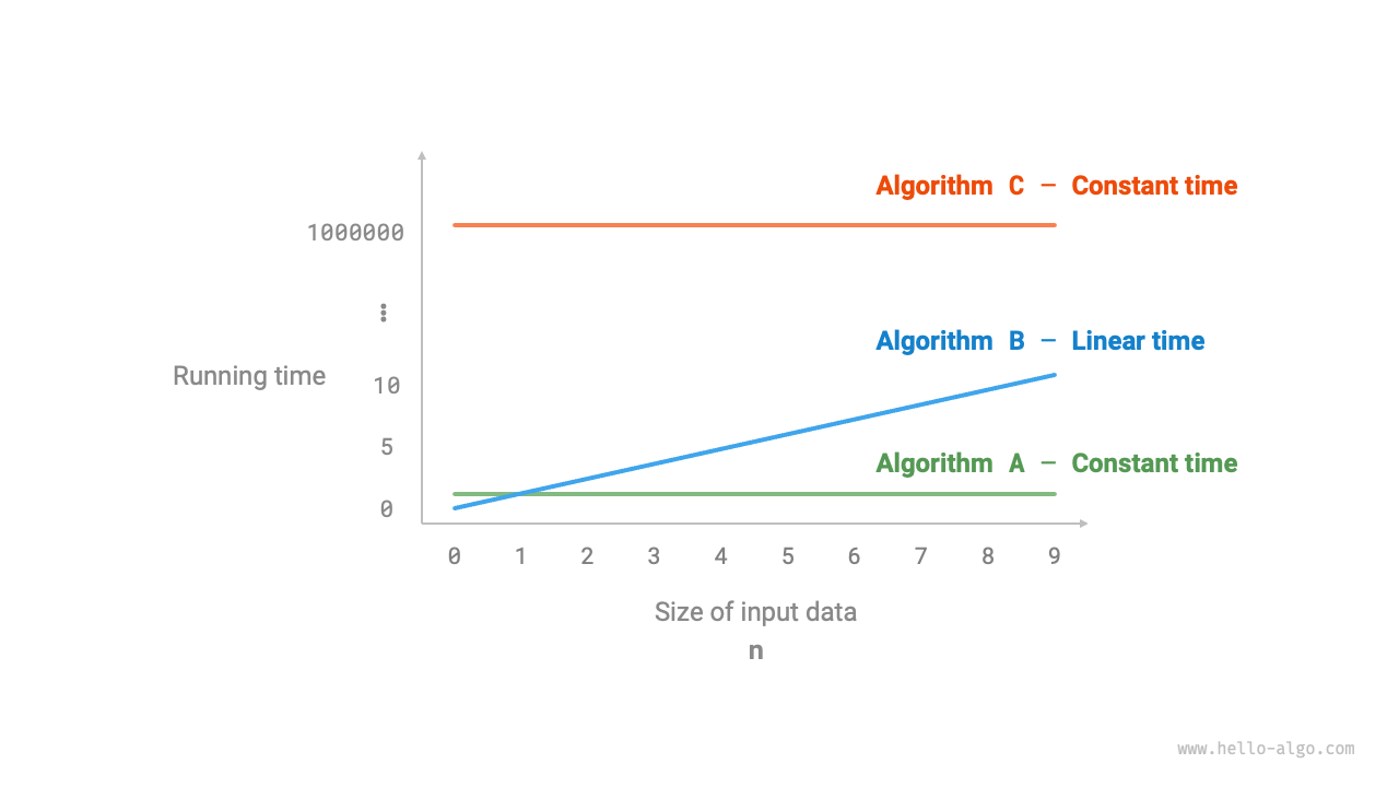
Figure 2-7 Time growth trends of algorithms A, B, and C
Compared to directly counting the algorithm's runtime, what are the characteristics of time complexity analysis?
- Time complexity can effectively evaluate algorithm efficiency. For example, the runtime of algorithm
Bgrows linearly; when \(n > 1\) it is slower than algorithmA, and when \(n > 1000000\) it is slower than algorithmC. In fact, as long as the input data size \(n\) is sufficiently large, an algorithm with "constant order" complexity will always be superior to one with "linear order" complexity, which is precisely the meaning of time growth trend. - The derivation method for time complexity is simpler. Obviously, the running platform and the types of computational operations are both unrelated to the growth trend of the algorithm's runtime. Therefore, in time complexity analysis, we can simply treat the execution time of all computational operations as the same "unit time", reducing "tracking the runtime of each operation" to "counting the number of operations", which greatly reduces the difficulty of estimation.
- Time complexity also has certain limitations. For example, although algorithms
AandChave the same time complexity, their actual runtimes differ significantly. Similarly, although algorithmBhas a higher time complexity thanC, when the input data size \(n\) is small, algorithmBis clearly superior to algorithmC. In such cases, it is often difficult to judge the efficiency of algorithms based solely on time complexity. Of course, despite the above issues, complexity analysis remains the most effective and commonly used method for evaluating algorithm efficiency.
2.3.2 Asymptotic Upper Bound of Functions
Given a function with input size \(n\):
Let the number of operations of the algorithm be a function of the input data size \(n\), denoted as \(T(n)\). Then the number of operations of the above function is:
\(T(n)\) is a linear function, indicating that its runtime growth trend is linear, and therefore its time complexity is linear order.
We denote the time complexity of linear order as \(O(n)\). This mathematical symbol is called big-\(O\) notation, representing the asymptotic upper bound of the function \(T(n)\).
Time complexity analysis essentially calculates the asymptotic upper bound of "the number of operations \(T(n)\)", which has a clear mathematical definition.
Asymptotic upper bound of functions
If there exist positive real numbers \(c\) and \(n_0\) such that for all \(n > n_0\), we have \(T(n) \leq c \cdot f(n)\), then \(f(n)\) can be considered as an asymptotic upper bound of \(T(n)\), denoted as \(T(n) = O(f(n))\).
As shown in Figure 2-8, calculating the asymptotic upper bound is to find a function \(f(n)\) such that when \(n\) tends to infinity, \(T(n)\) and \(f(n)\) are at the same growth level, differing only by a constant coefficient \(c\).
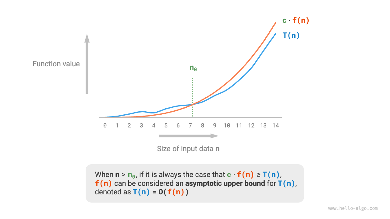
Figure 2-8 Asymptotic upper bound of a function
2.3.3 Derivation Method
The idea of an asymptotic upper bound is somewhat mathematical. If you feel you haven't fully understood it, don't worry. We can first master the derivation method, and gradually grasp its mathematical meaning through continuous practice.
According to the definition, after determining \(f(n)\), we can obtain the time complexity \(O(f(n))\). So how do we determine the asymptotic upper bound \(f(n)\)? Overall, it is divided into two steps: first count the number of operations, then determine the asymptotic upper bound.
1. Step 1: Count the Number of Operations
For code, count from top to bottom line by line. However, since the constant coefficient \(c\) in \(c \cdot f(n)\) above can be of any size, coefficients and constant terms in the number of operations \(T(n)\) can all be ignored. According to this principle, the following counting simplification techniques can be summarized.
- Ignore constants in \(T(n)\). Because they are all independent of \(n\), they do not affect time complexity.
- Omit all coefficients. For example, looping \(2n\) times, \(5n + 1\) times, etc., can all be simplified as \(n\) times, because the coefficient before \(n\) does not affect time complexity.
- Use multiplication for nested loops. The total number of operations equals the product of the number of operations in the outer and inner loops, with each layer of loop still able to apply techniques
1.and2.separately.
Given a function, we can use the above techniques to count the number of operations:
The following formula shows the counting results before and after using the above techniques; both derive a time complexity of \(O(n^2)\).
2. Step 2: Determine the Asymptotic Upper Bound
Time complexity is determined by the highest-order term in \(T(n)\). This is because as \(n\) tends to infinity, the highest-order term will play a dominant role, and the influence of other terms can be ignored.
Table 2-2 shows some examples, where some exaggerated values are used to emphasize the conclusion that "coefficients cannot shake the order". When \(n\) tends to infinity, these constants become insignificant.
Table 2-2 Time complexities corresponding to different numbers of operations
| Number of Operations \(T(n)\) | Time Complexity \(O(f(n))\) |
|---|---|
| \(100000\) | \(O(1)\) |
| \(3n + 2\) | \(O(n)\) |
| \(2n^2 + 3n + 2\) | \(O(n^2)\) |
| \(n^3 + 10000n^2\) | \(O(n^3)\) |
| \(2^n + 10000n^{10000}\) | \(O(2^n)\) |
2.3.4 Common Types
Let the input data size be \(n\). Common time complexity types are shown in Figure 2-9 (arranged in order from low to high).
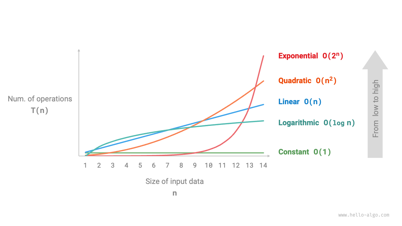
Figure 2-9 Common time complexity types
1. Constant Order \(O(1)\)
The number of operations in constant order is independent of the input data size \(n\), meaning it does not change as \(n\) changes.
In the following function, although the value of size may be large, it is independent of the input data size \(n\), so the time complexity remains \(O(1)\):
2. Linear Order \(O(n)\)
The number of operations in linear order grows linearly relative to the input data size \(n\). Linear order typically appears in single-layer loops:
Operations such as traversing arrays and traversing linked lists have a time complexity of \(O(n)\), where \(n\) is the length of the array or linked list:
It is worth noting that the input data size \(n\) should be determined according to the type of input data. For example, in the first example, the variable \(n\) is the input data size; in the second example, the array length \(n\) is the data size.
3. Quadratic Order \(O(n^2)\)
The number of operations in quadratic order grows quadratically relative to the input data size \(n\). Quadratic order typically appears in nested loops, where both the outer and inner loops have a time complexity of \(O(n)\), resulting in an overall time complexity of \(O(n^2)\):
Figure 2-10 compares constant order, linear order, and quadratic order time complexities.
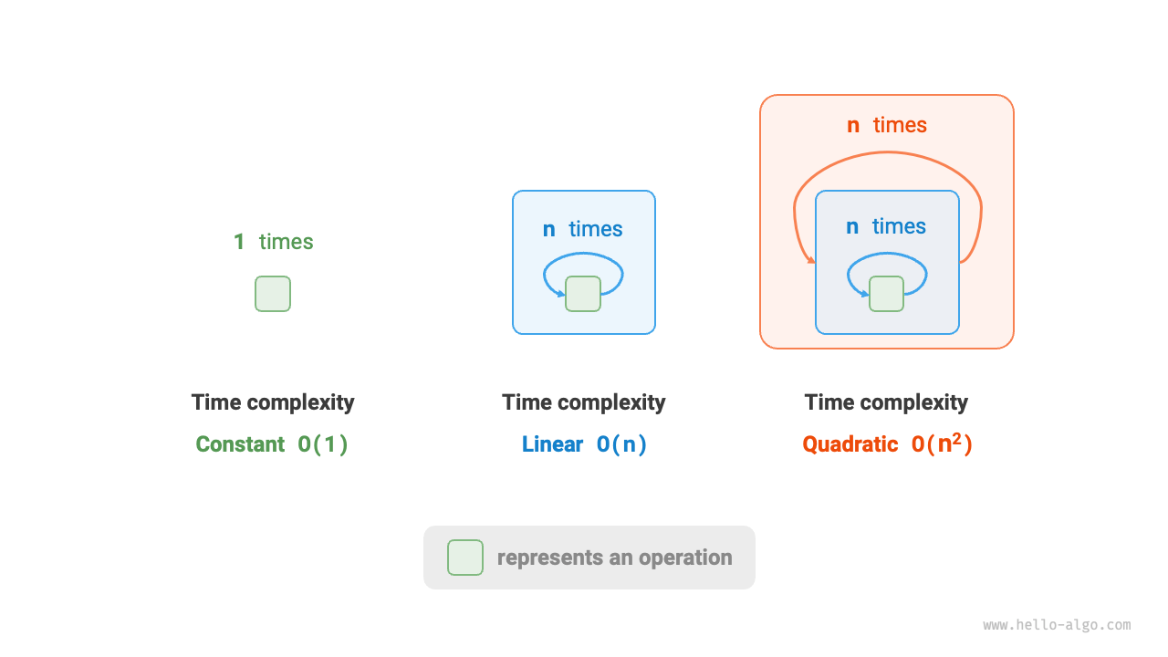
Figure 2-10 Time complexities of constant, linear, and quadratic orders
Taking bubble sort as an example, the outer loop executes \(n - 1\) times, and the inner loop executes \(n-1\), \(n-2\), \(\dots\), \(2\), \(1\) times, averaging \(n / 2\) times, resulting in a time complexity of \(O((n - 1) n / 2) = O(n^2)\):
def bubble_sort(nums: list[int]) -> int:
    """Quadratic order (bubble sort)"""
    count = 0  # Counter
    # Outer loop: unsorted range is [0, i]
    for i in range(len(nums) - 1, 0, -1):
        # Inner loop: swap the largest element in the unsorted range [0, i] to the rightmost end of that range
        for j in range(i):
            if nums[j] > nums[j + 1]:
                # Swap nums[j] and nums[j + 1]
                tmp: int = nums[j]
                nums[j] = nums[j + 1]
                nums[j + 1] = tmp
                count += 3  # Element swap includes 3 unit operations
    return count
/* Quadratic order (bubble sort) */
int bubbleSort(vector<int> &nums) {
    int count = 0; // Counter
    // Outer loop: unsorted range is [0, i]
    for (int i = nums.size() - 1; i > 0; i--) {
        // Inner loop: swap the largest element in the unsorted range [0, i] to the rightmost end of that range
        for (int j = 0; j < i; j++) {
            if (nums[j] > nums[j + 1]) {
                // Swap nums[j] and nums[j + 1]
                int tmp = nums[j];
                nums[j] = nums[j + 1];
                nums[j + 1] = tmp;
                count += 3; // Element swap includes 3 unit operations
            }
        }
    }
    return count;
}
/* Quadratic order (bubble sort) */
int bubbleSort(int[] nums) {
    int count = 0; // Counter
    // Outer loop: unsorted range is [0, i]
    for (int i = nums.length - 1; i > 0; i--) {
        // Inner loop: swap the largest element in the unsorted range [0, i] to the rightmost end of that range
        for (int j = 0; j < i; j++) {
            if (nums[j] > nums[j + 1]) {
                // Swap nums[j] and nums[j + 1]
                int tmp = nums[j];
                nums[j] = nums[j + 1];
                nums[j + 1] = tmp;
                count += 3; // Element swap includes 3 unit operations
            }
        }
    }
    return count;
}
/* Quadratic order (bubble sort) */
int BubbleSort(int[] nums) {
    int count = 0;  // Counter
    // Outer loop: unsorted range is [0, i]
    for (int i = nums.Length - 1; i > 0; i--) {
        // Inner loop: swap the largest element in the unsorted range [0, i] to the rightmost end of that range
        for (int j = 0; j < i; j++) {
            if (nums[j] > nums[j + 1]) {
                // Swap nums[j] and nums[j + 1]
                (nums[j + 1], nums[j]) = (nums[j], nums[j + 1]);
                count += 3;  // Element swap includes 3 unit operations
            }
        }
    }
    return count;
}
/* Quadratic order (bubble sort) */
func bubbleSort(nums []int) int {
    count := 0 // Counter
    // Outer loop: unsorted range is [0, i]
    for i := len(nums) - 1; i > 0; i-- {
        // Inner loop: swap the largest element in the unsorted range [0, i] to the rightmost end of that range
        for j := 0; j < i; j++ {
            if nums[j] > nums[j+1] {
                // Swap nums[j] and nums[j + 1]
                tmp := nums[j]
                nums[j] = nums[j+1]
                nums[j+1] = tmp
                count += 3 // Element swap includes 3 unit operations
            }
        }
    }
    return count
}
/* Quadratic order (bubble sort) */
func bubbleSort(nums: inout [Int]) -> Int {
    var count = 0 // Counter
    // Outer loop: unsorted range is [0, i]
    for i in nums.indices.dropFirst().reversed() {
        // Inner loop: swap the largest element in the unsorted range [0, i] to the rightmost end of that range
        for j in 0 ..< i {
            if nums[j] > nums[j + 1] {
                // Swap nums[j] and nums[j + 1]
                let tmp = nums[j]
                nums[j] = nums[j + 1]
                nums[j + 1] = tmp
                count += 3 // Element swap includes 3 unit operations
            }
        }
    }
    return count
}
/* Quadratic order (bubble sort) */
function bubbleSort(nums) {
    let count = 0; // Counter
    // Outer loop: unsorted range is [0, i]
    for (let i = nums.length - 1; i > 0; i--) {
        // Inner loop: swap the largest element in the unsorted range [0, i] to the rightmost end of that range
        for (let j = 0; j < i; j++) {
            if (nums[j] > nums[j + 1]) {
                // Swap nums[j] and nums[j + 1]
                let tmp = nums[j];
                nums[j] = nums[j + 1];
                nums[j + 1] = tmp;
                count += 3; // Element swap includes 3 unit operations
            }
        }
    }
    return count;
}
/* Quadratic order (bubble sort) */
function bubbleSort(nums: number[]): number {
    let count = 0; // Counter
    // Outer loop: unsorted range is [0, i]
    for (let i = nums.length - 1; i > 0; i--) {
        // Inner loop: swap the largest element in the unsorted range [0, i] to the rightmost end of that range
        for (let j = 0; j < i; j++) {
            if (nums[j] > nums[j + 1]) {
                // Swap nums[j] and nums[j + 1]
                let tmp = nums[j];
                nums[j] = nums[j + 1];
                nums[j + 1] = tmp;
                count += 3; // Element swap includes 3 unit operations
            }
        }
    }
    return count;
}
/* Quadratic order (bubble sort) */
int bubbleSort(List<int> nums) {
  int count = 0; // Counter
  // Outer loop: unsorted range is [0, i]
  for (var i = nums.length - 1; i > 0; i--) {
    // Inner loop: swap the largest element in the unsorted range [0, i] to the rightmost end of that range
    for (var j = 0; j < i; j++) {
      if (nums[j] > nums[j + 1]) {
        // Swap nums[j] and nums[j + 1]
        int tmp = nums[j];
        nums[j] = nums[j + 1];
        nums[j + 1] = tmp;
        count += 3; // Element swap includes 3 unit operations
      }
    }
  }
  return count;
}
/* Quadratic order (bubble sort) */
fn bubble_sort(nums: &mut [i32]) -> i32 {
    let mut count = 0; // Counter

    // Outer loop: unsorted range is [0, i]
    for i in (1..nums.len()).rev() {
        // Inner loop: swap the largest element in the unsorted range [0, i] to the rightmost end of that range
        for j in 0..i {
            if nums[j] > nums[j + 1] {
                // Swap nums[j] and nums[j + 1]
                let tmp = nums[j];
                nums[j] = nums[j + 1];
                nums[j + 1] = tmp;
                count += 3; // Element swap includes 3 unit operations
            }
        }
    }
    count
}
/* Quadratic order (bubble sort) */
int bubbleSort(int *nums, int n) {
    int count = 0; // Counter
    // Outer loop: unsorted range is [0, i]
    for (int i = n - 1; i > 0; i--) {
        // Inner loop: swap the largest element in the unsorted range [0, i] to the rightmost end of that range
        for (int j = 0; j < i; j++) {
            if (nums[j] > nums[j + 1]) {
                // Swap nums[j] and nums[j + 1]
                int tmp = nums[j];
                nums[j] = nums[j + 1];
                nums[j + 1] = tmp;
                count += 3; // Element swap includes 3 unit operations
            }
        }
    }
    return count;
}
/* Quadratic order (bubble sort) */
fun bubbleSort(nums: IntArray): Int {
    var count = 0 // Counter
    // Outer loop: unsorted range is [0, i]
    for (i in nums.size - 1 downTo 1) {
        // Inner loop: swap the largest element in the unsorted range [0, i] to the rightmost end of that range
        for (j in 0..<i) {
            if (nums[j] > nums[j + 1]) {
                // Swap nums[j] and nums[j + 1]
                val temp = nums[j]
                nums[j] = nums[j + 1]
                nums[j + 1] = temp
                count += 3 // Element swap includes 3 unit operations
            }
        }
    }
    return count
}
### Quadratic time (bubble sort) ###
def bubble_sort(nums)
  count = 0  # Counter

  # Outer loop: unsorted range is [0, i]
  for i in (nums.length - 1).downto(0)
    # Inner loop: swap the largest element in the unsorted range [0, i] to the rightmost end of that range
    for j in 0...i
      if nums[j] > nums[j + 1]
        # Swap nums[j] and nums[j + 1]
        tmp = nums[j]
        nums[j] = nums[j + 1]
        nums[j + 1] = tmp
        count += 3 # Element swap includes 3 unit operations
      end
    end
  end

  count
end
4. Exponential Order \(O(2^n)\)
Biological "cell division" is a typical example of exponential order growth: the initial state is \(1\) cell, after one round of division it becomes \(2\), after two rounds it becomes \(4\), and so on; after \(n\) rounds of division there are \(2^n\) cells.
Figure 2-11 and the following code simulate the cell division process, with a time complexity of \(O(2^n)\). Note that the input \(n\) represents the number of division rounds, and the return value count represents the total number of divisions.
def exponential(n: int) -> int:
    """Exponential order (loop implementation)"""
    count = 0
    base = 1
    # Cells divide into two every round, forming sequence 1, 2, 4, 8, ..., 2^(n-1)
    for _ in range(n):
        for _ in range(base):
            count += 1
        base *= 2
    # count = 1 + 2 + 4 + 8 + .. + 2^(n-1) = 2^n - 1
    return count
/* Exponential order (loop implementation) */
int exponential(int n) {
    int count = 0, base = 1;
    // Cells divide into two every round, forming sequence 1, 2, 4, 8, ..., 2^(n-1)
    for (int i = 0; i < n; i++) {
        for (int j = 0; j < base; j++) {
            count++;
        }
        base *= 2;
    }
    // count = 1 + 2 + 4 + 8 + .. + 2^(n-1) = 2^n - 1
    return count;
}
/* Exponential order (loop implementation) */
int Exponential(int n) {
    int count = 0, bas = 1;
    // Cells divide into two every round, forming sequence 1, 2, 4, 8, ..., 2^(n-1)
    for (int i = 0; i < n; i++) {
        for (int j = 0; j < bas; j++) {
            count++;
        }
        bas *= 2;
    }
    // count = 1 + 2 + 4 + 8 + .. + 2^(n-1) = 2^n - 1
    return count;
}
/* Exponential order (loop implementation) */
func exponential(n int) int {
    count, base := 0, 1
    // Cells divide into two every round, forming sequence 1, 2, 4, 8, ..., 2^(n-1)
    for i := 0; i < n; i++ {
        for j := 0; j < base; j++ {
            count++
        }
        base *= 2
    }
    // count = 1 + 2 + 4 + 8 + .. + 2^(n-1) = 2^n - 1
    return count
}
/* Exponential order (loop implementation) */
func exponential(n: Int) -> Int {
    var count = 0
    var base = 1
    // Cells divide into two every round, forming sequence 1, 2, 4, 8, ..., 2^(n-1)
    for _ in 0 ..< n {
        for _ in 0 ..< base {
            count += 1
        }
        base *= 2
    }
    // count = 1 + 2 + 4 + 8 + .. + 2^(n-1) = 2^n - 1
    return count
}
/* Exponential order (loop implementation) */
function exponential(n) {
    let count = 0,
        base = 1;
    // Cells divide into two every round, forming sequence 1, 2, 4, 8, ..., 2^(n-1)
    for (let i = 0; i < n; i++) {
        for (let j = 0; j < base; j++) {
            count++;
        }
        base *= 2;
    }
    // count = 1 + 2 + 4 + 8 + .. + 2^(n-1) = 2^n - 1
    return count;
}
/* Exponential order (loop implementation) */
function exponential(n: number): number {
    let count = 0,
        base = 1;
    // Cells divide into two every round, forming sequence 1, 2, 4, 8, ..., 2^(n-1)
    for (let i = 0; i < n; i++) {
        for (let j = 0; j < base; j++) {
            count++;
        }
        base *= 2;
    }
    // count = 1 + 2 + 4 + 8 + .. + 2^(n-1) = 2^n - 1
    return count;
}
/* Exponential order (loop implementation) */
int exponential(int n) {
  int count = 0, base = 1;
  // Cells divide into two every round, forming sequence 1, 2, 4, 8, ..., 2^(n-1)
  for (var i = 0; i < n; i++) {
    for (var j = 0; j < base; j++) {
      count++;
    }
    base *= 2;
  }
  // count = 1 + 2 + 4 + 8 + .. + 2^(n-1) = 2^n - 1
  return count;
}
/* Exponential order (loop implementation) */
fn exponential(n: i32) -> i32 {
    let mut count = 0;
    let mut base = 1;
    // Cells divide into two every round, forming sequence 1, 2, 4, 8, ..., 2^(n-1)
    for _ in 0..n {
        for _ in 0..base {
            count += 1
        }
        base *= 2;
    }
    // count = 1 + 2 + 4 + 8 + .. + 2^(n-1) = 2^n - 1
    count
}
/* Exponential order (loop implementation) */
int exponential(int n) {
    int count = 0;
    int bas = 1;
    // Cells divide into two every round, forming sequence 1, 2, 4, 8, ..., 2^(n-1)
    for (int i = 0; i < n; i++) {
        for (int j = 0; j < bas; j++) {
            count++;
        }
        bas *= 2;
    }
    // count = 1 + 2 + 4 + 8 + .. + 2^(n-1) = 2^n - 1
    return count;
}
/* Exponential order (loop implementation) */
fun exponential(n: Int): Int {
    var count = 0
    var base = 1
    // Cells divide into two every round, forming sequence 1, 2, 4, 8, ..., 2^(n-1)
    for (i in 0..<n) {
        for (j in 0..<base) {
            count++
        }
        base *= 2
    }
    // count = 1 + 2 + 4 + 8 + .. + 2^(n-1) = 2^n - 1
    return count
}
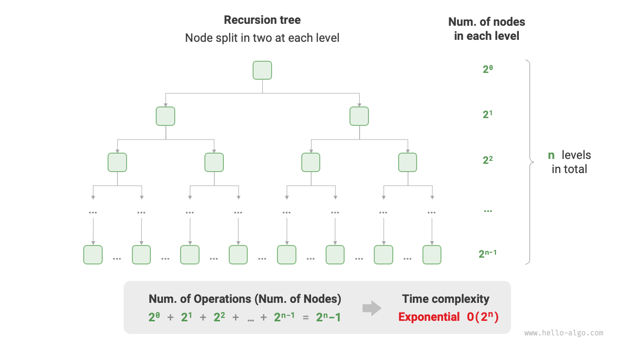
Figure 2-11 Time complexity of exponential order
In actual algorithms, exponential order often appears in recursive functions. For example, in the following code, it recursively splits in two, stopping after \(n\) splits:
Exponential order growth is very rapid and is common in exhaustive methods (brute force search, backtracking, etc.). For problems with large data scales, exponential order is unacceptable and typically requires dynamic programming or greedy algorithms to solve.
5. Logarithmic Order \(O(\log n)\)
In contrast to exponential order, logarithmic order reflects the situation of "reducing to half each round". Let the input data size be \(n\). Since it is reduced to half each round, the number of loops is \(\log_2 n\), which is the inverse function of \(2^n\).
Figure 2-12 and the following code simulate the process of "reducing to half each round", with a time complexity of \(O(\log_2 n)\), abbreviated as \(O(\log n)\):
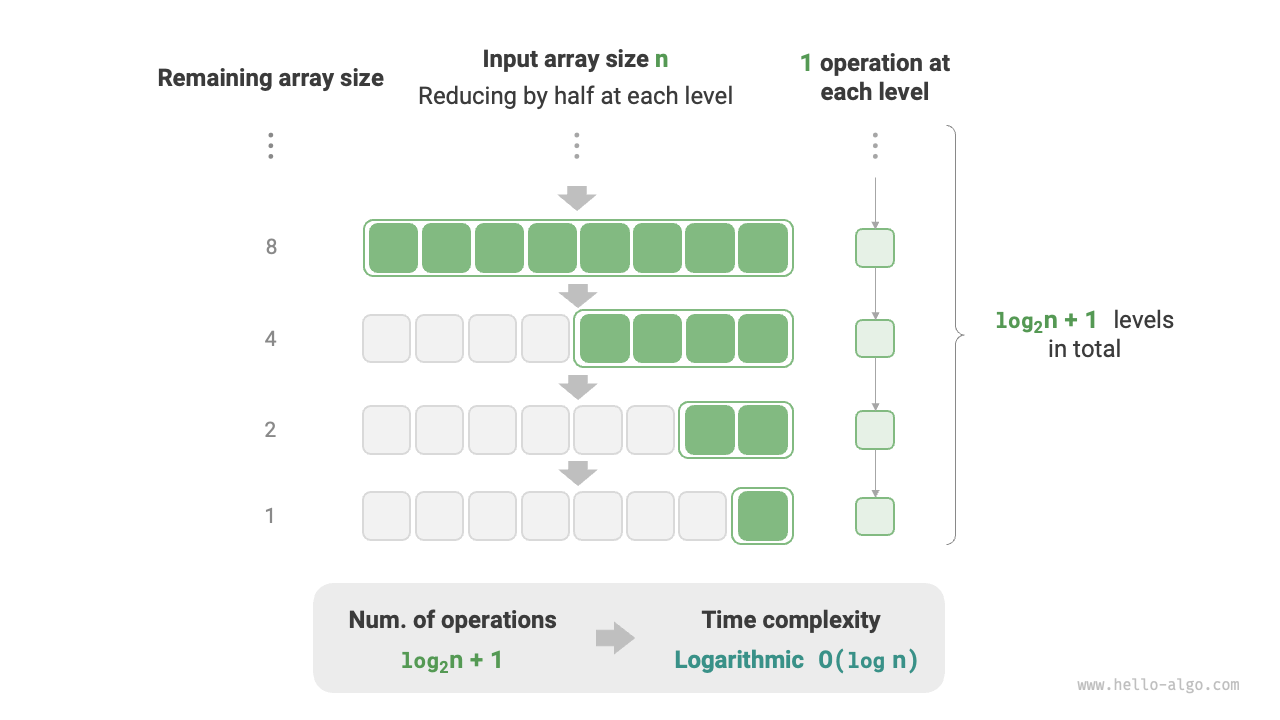
Figure 2-12 Time complexity of logarithmic order
Like exponential order, logarithmic order also commonly appears in recursive functions. The following code forms a recursion tree of height \(\log_2 n\):
Logarithmic order commonly appears in algorithms based on the divide-and-conquer strategy, reflecting the idea of repeatedly splitting a problem and simplifying it. It grows slowly and is the ideal time complexity second only to constant order.
What is the base of \(O(\log n)\)?
To be precise, "dividing into \(m\)" corresponds to a time complexity of \(O(\log_m n)\). And through the logarithmic base change formula, we can obtain time complexities with different bases that are equal:
That is to say, the base \(m\) can be converted without affecting the complexity. Therefore, we usually omit the base \(m\) and denote logarithmic order simply as \(O(\log n)\).
6. Linearithmic Order \(O(n \log n)\)
Linearithmic order commonly appears in nested loops, where the time complexities of the two layers of loops are \(O(\log n)\) and \(O(n)\) respectively. The relevant code is as follows:
def linear_log_recur(n: int) -> int:
    """Linearithmic order"""
    if n <= 1:
        return 1
    # Divide into two, the scale of subproblems is reduced by half
    count = linear_log_recur(n // 2) + linear_log_recur(n // 2)
    # Current subproblem contains n operations
    for _ in range(n):
        count += 1
    return count
Figure 2-13 shows how linearithmic order is generated. Each level of the binary tree has a total of \(n\) operations, and the tree has \(\log_2 n + 1\) levels, resulting in a time complexity of \(O(n \log n)\).
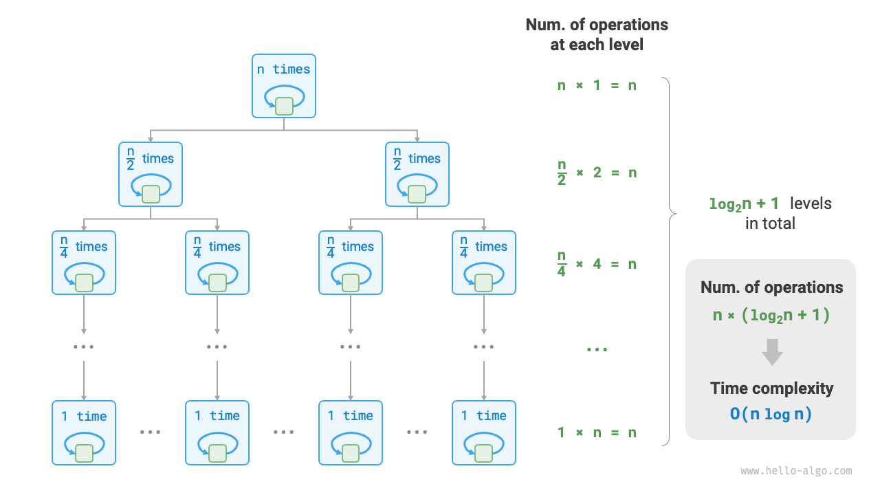
Figure 2-13 Time complexity of linearithmic order
Mainstream sorting algorithms typically have a time complexity of \(O(n \log n)\), such as quicksort, merge sort, and heap sort.
7. Factorial Order \(O(n!)\)
Factorial order corresponds to the mathematical "permutation" problem. Given \(n\) distinct elements, find all possible permutation schemes; the number of schemes is:
Factorials are typically implemented using recursion. As shown in Figure 2-14 and the following code, the first level splits into \(n\) branches, the second level splits into \(n - 1\) branches, and so on, until the \(n\)-th level when splitting stops:
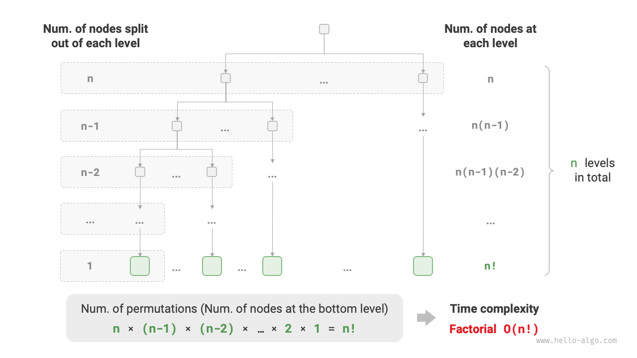
Figure 2-14 Time complexity of factorial order
Note that because when \(n \geq 4\) we always have \(n! > 2^n\), factorial order grows faster than exponential order, and is also unacceptable for large \(n\).
2.3.5 Worst, Best, and Average Time Complexities
The time efficiency of an algorithm is often not fixed, but is related to the distribution of the input data. Suppose we input an array nums of length \(n\), where nums consists of numbers from \(1\) to \(n\), with each number appearing only once, but the element order is randomly shuffled. The task is to return the index of element \(1\). We can draw the following conclusions.
- When
nums = [?, ?, ..., 1], i.e., when the last element is \(1\), it requires a complete traversal of the array, reaching worst-case time complexity \(O(n)\). - When
nums = [1, ?, ?, ...], i.e., when the first element is \(1\), no matter how long the array is, there is no need to continue traversing, reaching best-case time complexity \(\Omega(1)\).
The "worst-case time complexity" corresponds to the function's asymptotic upper bound, denoted using big-\(O\) notation. Correspondingly, the "best-case time complexity" corresponds to the function's asymptotic lower bound, denoted using \(\Omega\) notation:
def random_numbers(n: int) -> list[int]:
    """Generate an array with elements: 1, 2, ..., n, shuffled in order"""
    # Generate array nums =: 1, 2, 3, ..., n
    nums = [i for i in range(1, n + 1)]
    # Randomly shuffle array elements
    random.shuffle(nums)
    return nums

def find_one(nums: list[int]) -> int:
    """Find the index of number 1 in array nums"""
    for i in range(len(nums)):
        # When element 1 is at the head of the array, best time complexity O(1) is achieved
        # When element 1 is at the tail of the array, worst time complexity O(n) is achieved
        if nums[i] == 1:
            return i
    return -1
/* Generate an array with elements { 1, 2, ..., n }, order shuffled */
vector<int> randomNumbers(int n) {
    vector<int> nums(n);
    // Generate array nums = { 1, 2, 3, ..., n }
    for (int i = 0; i < n; i++) {
        nums[i] = i + 1;
    }
    // Use system time to generate random seed
    unsigned seed = chrono::system_clock::now().time_since_epoch().count();
    // Randomly shuffle array elements
    shuffle(nums.begin(), nums.end(), default_random_engine(seed));
    return nums;
}

/* Find the index of number 1 in array nums */
int findOne(vector<int> &nums) {
    for (int i = 0; i < nums.size(); i++) {
        // When element 1 is at the head of the array, best time complexity O(1) is achieved
        // When element 1 is at the tail of the array, worst time complexity O(n) is achieved
        if (nums[i] == 1)
            return i;
    }
    return -1;
}
/* Generate an array with elements { 1, 2, ..., n }, order shuffled */
int[] randomNumbers(int n) {
    Integer[] nums = new Integer[n];
    // Generate array nums = { 1, 2, 3, ..., n }
    for (int i = 0; i < n; i++) {
        nums[i] = i + 1;
    }
    // Randomly shuffle array elements
    Collections.shuffle(Arrays.asList(nums));
    // Integer[] -> int[]
    int[] res = new int[n];
    for (int i = 0; i < n; i++) {
        res[i] = nums[i];
    }
    return res;
}

/* Find the index of number 1 in array nums */
int findOne(int[] nums) {
    for (int i = 0; i < nums.length; i++) {
        // When element 1 is at the head of the array, best time complexity O(1) is achieved
        // When element 1 is at the tail of the array, worst time complexity O(n) is achieved
        if (nums[i] == 1)
            return i;
    }
    return -1;
}
/* Generate an array with elements { 1, 2, ..., n }, order shuffled */
int[] RandomNumbers(int n) {
    int[] nums = new int[n];
    // Generate array nums = { 1, 2, 3, ..., n }
    for (int i = 0; i < n; i++) {
        nums[i] = i + 1;
    }

    // Randomly shuffle array elements
    for (int i = 0; i < nums.Length; i++) {
        int index = new Random().Next(i, nums.Length);
        (nums[i], nums[index]) = (nums[index], nums[i]);
    }
    return nums;
}

/* Find the index of number 1 in array nums */
int FindOne(int[] nums) {
    for (int i = 0; i < nums.Length; i++) {
        // When element 1 is at the head of the array, best time complexity O(1) is achieved
        // When element 1 is at the tail of the array, worst time complexity O(n) is achieved
        if (nums[i] == 1)
            return i;
    }
    return -1;
}
/* Generate an array with elements { 1, 2, ..., n }, order shuffled */
func randomNumbers(n int) []int {
    nums := make([]int, n)
    // Generate array nums = { 1, 2, 3, ..., n }
    for i := 0; i < n; i++ {
        nums[i] = i + 1
    }
    // Randomly shuffle array elements
    rand.Shuffle(len(nums), func(i, j int) {
        nums[i], nums[j] = nums[j], nums[i]
    })
    return nums
}

/* Find the index of number 1 in array nums */
func findOne(nums []int) int {
    for i := 0; i < len(nums); i++ {
        // When element 1 is at the head of the array, best time complexity O(1) is achieved
        // When element 1 is at the tail of the array, worst time complexity O(n) is achieved
        if nums[i] == 1 {
            return i
        }
    }
    return -1
}
/* Generate an array with elements { 1, 2, ..., n }, order shuffled */
func randomNumbers(n: Int) -> [Int] {
// Generate array nums = { 1, 2, 3, ..., n }
var nums = Array(1 ... n)
// Randomly shuffle array elements
nums.shuffle()
return nums
}
/* Find the index of number 1 in array nums */
func findOne(nums: [Int]) -> Int {
for i in nums.indices {
// When element 1 is at the head of the array, best time complexity O(1) is achieved
// When element 1 is at the tail of the array, worst time complexity O(n) is achieved
if nums[i] == 1 {
return i
}
}
return -1
}
/* Generate an array with elements { 1, 2, ..., n }, order shuffled */
function randomNumbers(n) {
const nums = Array(n);
// Generate array nums = { 1, 2, 3, ..., n }
for (let i = 0; i < n; i++) {
nums[i] = i + 1;
}
// Randomly shuffle array elements
for (let i = 0; i < n; i++) {
const r = Math.floor(Math.random() * (i + 1));
const temp = nums[i];
nums[i] = nums[r];
nums[r] = temp;
}
return nums;
}
/* Find the index of number 1 in array nums */
function findOne(nums) {
for (let i = 0; i < nums.length; i++) {
// When element 1 is at the head of the array, best time complexity O(1) is achieved
// When element 1 is at the tail of the array, worst time complexity O(n) is achieved
if (nums[i] === 1) {
return i;
}
}
return -1;
}
/* Generate an array with elements { 1, 2, ..., n }, order shuffled */
function randomNumbers(n: number): number[] {
const nums = Array(n);
// Generate array nums = { 1, 2, 3, ..., n }
for (let i = 0; i < n; i++) {
nums[i] = i + 1;
}
// Randomly shuffle array elements
for (let i = 0; i < n; i++) {
const r = Math.floor(Math.random() * (i + 1));
const temp = nums[i];
nums[i] = nums[r];
nums[r] = temp;
}
return nums;
}
/* Find the index of number 1 in array nums */
function findOne(nums: number[]): number {
for (let i = 0; i < nums.length; i++) {
// When element 1 is at the head of the array, best time complexity O(1) is achieved
// When element 1 is at the tail of the array, worst time complexity O(n) is achieved
if (nums[i] === 1) {
return i;
}
}
return -1;
}
/* Generate an array with elements { 1, 2, ..., n }, order shuffled */
List<int> randomNumbers(int n) {
final nums = List.filled(n, 0);
// Generate array nums = { 1, 2, 3, ..., n }
for (var i = 0; i < n; i++) {
nums[i] = i + 1;
}
// Randomly shuffle array elements
nums.shuffle();
return nums;
}
/* Find the index of number 1 in array nums */
int findOne(List<int> nums) {
for (var i = 0; i < nums.length; i++) {
// When element 1 is at the head of the array, best time complexity O(1) is achieved
// When element 1 is at the tail of the array, worst time complexity O(n) is achieved
if (nums[i] == 1) return i;
}
return -1;
}
/* Generate an array with elements { 1, 2, ..., n }, order shuffled */
fn random_numbers(n: i32) -> Vec<i32> {
// Generate array nums = { 1, 2, 3, ..., n }
let mut nums = (1..=n).collect::<Vec<i32>>();
// Randomly shuffle array elements
nums.shuffle(&mut thread_rng());
nums
}
/* Find the index of number 1 in array nums */
fn find_one(nums: &[i32]) -> Option<usize> {
for i in 0..nums.len() {
// When element 1 is at the head of the array, best time complexity O(1) is achieved
// When element 1 is at the tail of the array, worst time complexity O(n) is achieved
if nums[i] == 1 {
return Some(i);
}
}
None
}
/* Generate an array with elements { 1, 2, ..., n }, order shuffled */
int *randomNumbers(int n) {
// Allocate heap memory (create 1D variable-length array: n elements of type int)
int *nums = (int *)malloc(n * sizeof(int));
// Generate array nums = { 1, 2, 3, ..., n }
for (int i = 0; i < n; i++) {
nums[i] = i + 1;
}
// Randomly shuffle array elements
for (int i = n - 1; i > 0; i--) {
int j = rand() % (i + 1);
int temp = nums[i];
nums[i] = nums[j];
nums[j] = temp;
}
return nums;
}
/* Find the index of number 1 in array nums */
int findOne(int *nums, int n) {
for (int i = 0; i < n; i++) {
// When element 1 is at the head of the array, best time complexity O(1) is achieved
// When element 1 is at the tail of the array, worst time complexity O(n) is achieved
if (nums[i] == 1)
return i;
}
return -1;
}
/* Generate an array with elements { 1, 2, ..., n }, order shuffled */
fun randomNumbers(n: Int): Array<Int?> {
val nums = IntArray(n)
// Generate array nums = { 1, 2, 3, ..., n }
for (i in 0..<n) {
nums[i] = i + 1
}
// Randomly shuffle array elements
nums.shuffle()
val res = arrayOfNulls<Int>(n)
for (i in 0..<n) {
res[i] = nums[i]
}
return res
}
/* Find the index of number 1 in array nums */
fun findOne(nums: Array<Int?>): Int {
for (i in nums.indices) {
// When element 1 is at the head of the array, best time complexity O(1) is achieved
// When element 1 is at the tail of the array, worst time complexity O(n) is achieved
if (nums[i] == 1)
return i
}
return -1
}
### Generate array with elements: 1, 2, ..., n, shuffled ###
def random_numbers(n)
# Generate array nums =: 1, 2, 3, ..., n
nums = Array.new(n) { |i| i + 1 }
# Randomly shuffle array elements
nums.shuffle!
end
### Find index of number 1 in array nums ###
def find_one(nums)
for i in 0...nums.length
# When element 1 is at the head of the array, best time complexity O(1) is achieved
# When element 1 is at the tail of the array, worst time complexity O(n) is achieved
return i if nums[i] == 1
end
-1
end
It is worth noting that we rarely use best-case time complexity in practice, because it can usually only be achieved with a very small probability and may be somewhat misleading. The worst-case time complexity is more practical because it gives a safety value for efficiency, allowing us to use the algorithm with confidence.
From the above example, we can see that both worst-case and best-case time complexities arise only under particular input distributions, which may occur with very low probability and may not truly reflect the algorithm's running efficiency. In contrast, average time complexity can reflect the algorithm's running efficiency under random input data, denoted using the \(\Theta\) notation.
For some algorithms, we can simply derive the average case under random data distribution. For example, in the above example, since the input array is shuffled, the probability of element \(1\) appearing at any index is equal, so the algorithm's average number of loops is half the array length \(n / 2\), giving an average time complexity of \(\Theta(n / 2) = \Theta(n)\).
But for more complex algorithms, calculating average time complexity is often quite difficult, because it is hard to analyze the overall mathematical expectation under data distribution. In this case, we usually use worst-case time complexity as the criterion for judging algorithm efficiency.
Why is the \(\Theta\) symbol rarely seen?
This may be because the \(O\) symbol is too catchy, so we often use it to represent average time complexity. But strictly speaking, this practice is not standard. In this book and other materials, if you encounter expressions like "average time complexity \(O(n)\)", please understand it directly as \(\Theta(n)\).