14.2 Characteristics of Dynamic Programming Problems
In the previous section, we learned how dynamic programming solves the original problem by decomposing it into subproblems. In fact, subproblem decomposition is a general algorithmic approach, with different emphases in divide and conquer, dynamic programming, and backtracking.
- Divide and conquer algorithms recursively divide the original problem into multiple independent subproblems until the smallest subproblems are reached, and merge the solutions to the subproblems during backtracking to ultimately obtain the solution to the original problem.
- Dynamic programming also recursively decomposes problems, but the main difference from divide and conquer algorithms is that subproblems in dynamic programming are interdependent, and many overlapping subproblems appear during the decomposition process.
- Backtracking algorithms enumerate all possible solutions through trial and error, and avoid unnecessary search branches through pruning. The solution to the original problem consists of a series of decision steps, and we can regard the subsequence before each decision step as a subproblem.
In fact, dynamic programming is commonly used to solve optimization problems, which not only contain overlapping subproblems but also have two other major characteristics: optimal substructure and no aftereffects.
14.2.1 Optimal Substructure
We make a slight modification to the stair climbing problem to make it more suitable for demonstrating the concept of optimal substructure.
Climbing stairs with minimum cost
Given a staircase, you can climb \(1\) or \(2\) steps at a time, and each step is labeled with a non-negative integer representing the cost of stepping on it. Given a non-negative integer array \(cost\), where \(cost[i]\) represents the cost of the \(i\)-th step and \(cost[0]\) is the ground (starting point), what is the minimum cost required to reach the top?
As shown in Figure 14-6, if the costs of the \(1\)st, \(2\)nd, and \(3\)rd steps are \(1\), \(10\), and \(1\) respectively, then climbing from the ground to the \(3\)rd step requires a minimum cost of \(2\).
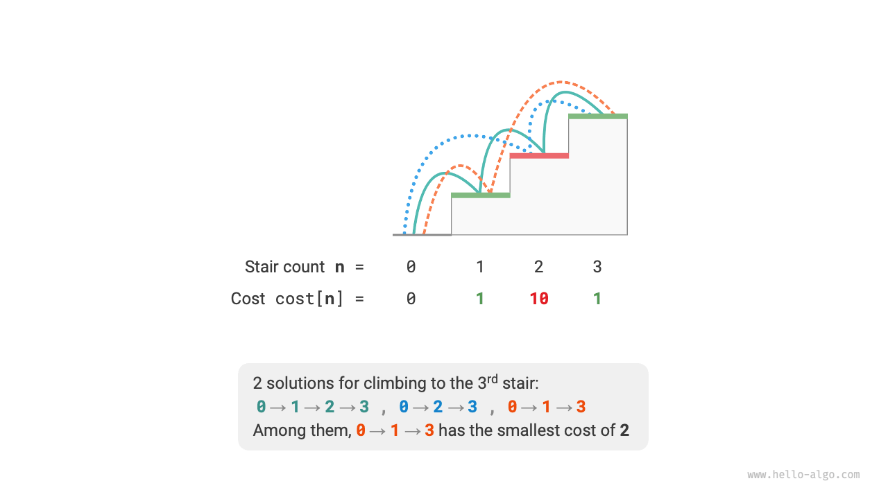
Figure 14-6 Minimum cost to climb to the 3rd step
Let \(dp[i]\) be the accumulated cost of climbing to the \(i\)-th step. Since the \(i\)-th step can only come from the \(i-1\)-th or \(i-2\)-th step, \(dp[i]\) can only equal \(dp[i-1] + cost[i]\) or \(dp[i-2] + cost[i]\). To minimize the cost, we should choose the smaller of the two:
This leads us to the meaning of optimal substructure: the optimal solution to the original problem is constructed from the optimal solutions to the subproblems.
This problem clearly has optimal substructure: we select the better one from the optimal solutions to the two subproblems \(dp[i-1]\) and \(dp[i-2]\), and use it to construct the optimal solution to the original problem \(dp[i]\).
So, does the stair climbing problem from the previous section have optimal substructure? Its goal is to find the number of ways, which seems to be a counting problem, but if we change the question: "Find the maximum number of ways". We surprisingly discover that although the problem before and after modification are equivalent, the optimal substructure has emerged: the maximum number of ways for the \(n\)-th step equals the sum of the maximum number of ways for the \(n-1\)-th and \(n-2\)-th steps. Therefore, the interpretation of optimal substructure is quite flexible and will have different meanings in different problems.
According to the state transition equation and the initial states \(dp[1] = cost[1]\) and \(dp[2] = cost[2]\), we can obtain the dynamic programming code:
def min_cost_climbing_stairs_dp(cost: list[int]) -> int:
    """Minimum cost climbing stairs: Dynamic programming"""
    n = len(cost) - 1
    if n == 1 or n == 2:
        return cost[n]
    # Initialize dp table, used to store solutions to subproblems
    dp = [0] * (n + 1)
    # Initial state: preset the solution to the smallest subproblem
    dp[1], dp[2] = cost[1], cost[2]
    # State transition: gradually solve larger subproblems from smaller ones
    for i in range(3, n + 1):
        dp[i] = min(dp[i - 1], dp[i - 2]) + cost[i]
    return dp[n]
/* Minimum cost climbing stairs: Dynamic programming */
int minCostClimbingStairsDP(vector<int> &cost) {
    int n = cost.size() - 1;
    if (n == 1 || n == 2)
        return cost[n];
    // Initialize dp table, used to store solutions to subproblems
    vector<int> dp(n + 1);
    // Initial state: preset the solution to the smallest subproblem
    dp[1] = cost[1];
    dp[2] = cost[2];
    // State transition: gradually solve larger subproblems from smaller ones
    for (int i = 3; i <= n; i++) {
        dp[i] = min(dp[i - 1], dp[i - 2]) + cost[i];
    }
    return dp[n];
}
/* Minimum cost climbing stairs: Dynamic programming */
int minCostClimbingStairsDP(int[] cost) {
    int n = cost.length - 1;
    if (n == 1 || n == 2)
        return cost[n];
    // Initialize dp table, used to store solutions to subproblems
    int[] dp = new int[n + 1];
    // Initial state: preset the solution to the smallest subproblem
    dp[1] = cost[1];
    dp[2] = cost[2];
    // State transition: gradually solve larger subproblems from smaller ones
    for (int i = 3; i <= n; i++) {
        dp[i] = Math.min(dp[i - 1], dp[i - 2]) + cost[i];
    }
    return dp[n];
}
/* Minimum cost climbing stairs: Dynamic programming */
int MinCostClimbingStairsDP(int[] cost) {
    int n = cost.Length - 1;
    if (n == 1 || n == 2)
        return cost[n];
    // Initialize dp table, used to store solutions to subproblems
    int[] dp = new int[n + 1];
    // Initial state: preset the solution to the smallest subproblem
    dp[1] = cost[1];
    dp[2] = cost[2];
    // State transition: gradually solve larger subproblems from smaller ones
    for (int i = 3; i <= n; i++) {
        dp[i] = Math.Min(dp[i - 1], dp[i - 2]) + cost[i];
    }
    return dp[n];
}
/* Minimum cost climbing stairs: Dynamic programming */
func minCostClimbingStairsDP(cost []int) int {
    n := len(cost) - 1
    if n == 1 || n == 2 {
        return cost[n]
    }
    min := func(a, b int) int {
        if a < b {
            return a
        }
        return b
    }
    // Initialize dp table, used to store solutions to subproblems
    dp := make([]int, n+1)
    // Initial state: preset the solution to the smallest subproblem
    dp[1] = cost[1]
    dp[2] = cost[2]
    // State transition: gradually solve larger subproblems from smaller ones
    for i := 3; i <= n; i++ {
        dp[i] = min(dp[i-1], dp[i-2]) + cost[i]
    }
    return dp[n]
}
/* Minimum cost climbing stairs: Dynamic programming */
func minCostClimbingStairsDP(cost: [Int]) -> Int {
    let n = cost.count - 1
    if n == 1 || n == 2 {
        return cost[n]
    }
    // Initialize dp table, used to store solutions to subproblems
    var dp = Array(repeating: 0, count: n + 1)
    // Initial state: preset the solution to the smallest subproblem
    dp[1] = cost[1]
    dp[2] = cost[2]
    // State transition: gradually solve larger subproblems from smaller ones
    for i in 3 ... n {
        dp[i] = min(dp[i - 1], dp[i - 2]) + cost[i]
    }
    return dp[n]
}
/* Minimum cost climbing stairs: Dynamic programming */
function minCostClimbingStairsDP(cost) {
    const n = cost.length - 1;
    if (n === 1 || n === 2) {
        return cost[n];
    }
    // Initialize dp table, used to store solutions to subproblems
    const dp = new Array(n + 1);
    // Initial state: preset the solution to the smallest subproblem
    dp[1] = cost[1];
    dp[2] = cost[2];
    // State transition: gradually solve larger subproblems from smaller ones
    for (let i = 3; i <= n; i++) {
        dp[i] = Math.min(dp[i - 1], dp[i - 2]) + cost[i];
    }
    return dp[n];
}
/* Minimum cost climbing stairs: Dynamic programming */
function minCostClimbingStairsDP(cost: Array<number>): number {
    const n = cost.length - 1;
    if (n === 1 || n === 2) {
        return cost[n];
    }
    // Initialize dp table, used to store solutions to subproblems
    const dp = new Array(n + 1);
    // Initial state: preset the solution to the smallest subproblem
    dp[1] = cost[1];
    dp[2] = cost[2];
    // State transition: gradually solve larger subproblems from smaller ones
    for (let i = 3; i <= n; i++) {
        dp[i] = Math.min(dp[i - 1], dp[i - 2]) + cost[i];
    }
    return dp[n];
}
/* Minimum cost climbing stairs: Dynamic programming */
int minCostClimbingStairsDP(List<int> cost) {
  int n = cost.length - 1;
  if (n == 1 || n == 2) return cost[n];
  // Initialize dp table, used to store solutions to subproblems
  List<int> dp = List.filled(n + 1, 0);
  // Initial state: preset the solution to the smallest subproblem
  dp[1] = cost[1];
  dp[2] = cost[2];
  // State transition: gradually solve larger subproblems from smaller ones
  for (int i = 3; i <= n; i++) {
    dp[i] = min(dp[i - 1], dp[i - 2]) + cost[i];
  }
  return dp[n];
}
/* Minimum cost climbing stairs: Dynamic programming */
fn min_cost_climbing_stairs_dp(cost: &[i32]) -> i32 {
    let n = cost.len() - 1;
    if n == 1 || n == 2 {
        return cost[n];
    }
    // Initialize dp table, used to store solutions to subproblems
    let mut dp = vec![-1; n + 1];
    // Initial state: preset the solution to the smallest subproblem
    dp[1] = cost[1];
    dp[2] = cost[2];
    // State transition: gradually solve larger subproblems from smaller ones
    for i in 3..=n {
        dp[i] = cmp::min(dp[i - 1], dp[i - 2]) + cost[i];
    }
    dp[n]
}
/* Minimum cost climbing stairs: Dynamic programming */
int minCostClimbingStairsDP(int cost[], int costSize) {
    int n = costSize - 1;
    if (n == 1 || n == 2)
        return cost[n];
    // Initialize dp table, used to store solutions to subproblems
    int *dp = calloc(n + 1, sizeof(int));
    // Initial state: preset the solution to the smallest subproblem
    dp[1] = cost[1];
    dp[2] = cost[2];
    // State transition: gradually solve larger subproblems from smaller ones
    for (int i = 3; i <= n; i++) {
        dp[i] = myMin(dp[i - 1], dp[i - 2]) + cost[i];
    }
    int res = dp[n];
    // Free memory
    free(dp);
    return res;
}
/* Minimum cost climbing stairs: Dynamic programming */
fun minCostClimbingStairsDP(cost: IntArray): Int {
    val n = cost.size - 1
    if (n == 1 || n == 2) return cost[n]
    // Initialize dp table, used to store solutions to subproblems
    val dp = IntArray(n + 1)
    // Initial state: preset the solution to the smallest subproblem
    dp[1] = cost[1]
    dp[2] = cost[2]
    // State transition: gradually solve larger subproblems from smaller ones
    for (i in 3..n) {
        dp[i] = min(dp[i - 1], dp[i - 2]) + cost[i]
    }
    return dp[n]
}
### Minimum cost climbing stairs: DP ###
def min_cost_climbing_stairs_dp(cost)
  n = cost.length - 1
  return cost[n] if n == 1 || n == 2
  # Initialize dp table, used to store solutions to subproblems
  dp = Array.new(n + 1, 0)
  # Initial state: preset the solution to the smallest subproblem
  dp[1], dp[2] = cost[1], cost[2]
  # State transition: gradually solve larger subproblems from smaller ones
  (3...(n + 1)).each { |i| dp[i] = [dp[i - 1], dp[i - 2]].min + cost[i] }
  dp[n]
end
Figure 14-7 shows the dynamic programming process for the above code.

Figure 14-7 Dynamic programming process for climbing stairs with minimum cost
This problem can also be space-optimized, compressing from one dimension to zero, reducing the space complexity from \(O(n)\) to \(O(1)\):
def min_cost_climbing_stairs_dp_comp(cost: list[int]) -> int:
    """Minimum cost climbing stairs: Space-optimized dynamic programming"""
    n = len(cost) - 1
    if n == 1 or n == 2:
        return cost[n]
    a, b = cost[1], cost[2]
    for i in range(3, n + 1):
        a, b = b, min(a, b) + cost[i]
    return b
/* Minimum cost climbing stairs: Space-optimized dynamic programming */
int minCostClimbingStairsDPComp(vector<int> &cost) {
    int n = cost.size() - 1;
    if (n == 1 || n == 2)
        return cost[n];
    int a = cost[1], b = cost[2];
    for (int i = 3; i <= n; i++) {
        int tmp = b;
        b = min(a, tmp) + cost[i];
        a = tmp;
    }
    return b;
}
/* Minimum cost climbing stairs: Space-optimized dynamic programming */
int minCostClimbingStairsDPComp(int[] cost) {
    int n = cost.length - 1;
    if (n == 1 || n == 2)
        return cost[n];
    int a = cost[1], b = cost[2];
    for (int i = 3; i <= n; i++) {
        int tmp = b;
        b = Math.min(a, tmp) + cost[i];
        a = tmp;
    }
    return b;
}
/* Minimum cost climbing stairs: Space-optimized dynamic programming */
int MinCostClimbingStairsDPComp(int[] cost) {
    int n = cost.Length - 1;
    if (n == 1 || n == 2)
        return cost[n];
    int a = cost[1], b = cost[2];
    for (int i = 3; i <= n; i++) {
        int tmp = b;
        b = Math.Min(a, tmp) + cost[i];
        a = tmp;
    }
    return b;
}
/* Minimum cost climbing stairs: Space-optimized dynamic programming */
func minCostClimbingStairsDPComp(cost []int) int {
    n := len(cost) - 1
    if n == 1 || n == 2 {
        return cost[n]
    }
    min := func(a, b int) int {
        if a < b {
            return a
        }
        return b
    }
    // Initial state: preset the solution to the smallest subproblem
    a, b := cost[1], cost[2]
    // State transition: gradually solve larger subproblems from smaller ones
    for i := 3; i <= n; i++ {
        tmp := b
        b = min(a, tmp) + cost[i]
        a = tmp
    }
    return b
}
/* Minimum cost climbing stairs: Space-optimized dynamic programming */
func minCostClimbingStairsDPComp(cost: [Int]) -> Int {
    let n = cost.count - 1
    if n == 1 || n == 2 {
        return cost[n]
    }
    var (a, b) = (cost[1], cost[2])
    for i in 3 ... n {
        (a, b) = (b, min(a, b) + cost[i])
    }
    return b
}
/* Minimum cost climbing stairs: Space-optimized dynamic programming */
function minCostClimbingStairsDPComp(cost) {
    const n = cost.length - 1;
    if (n === 1 || n === 2) {
        return cost[n];
    }
    let a = cost[1],
        b = cost[2];
    for (let i = 3; i <= n; i++) {
        const tmp = b;
        b = Math.min(a, tmp) + cost[i];
        a = tmp;
    }
    return b;
}
/* Minimum cost climbing stairs: Space-optimized dynamic programming */
function minCostClimbingStairsDPComp(cost: Array<number>): number {
    const n = cost.length - 1;
    if (n === 1 || n === 2) {
        return cost[n];
    }
    let a = cost[1],
        b = cost[2];
    for (let i = 3; i <= n; i++) {
        const tmp = b;
        b = Math.min(a, tmp) + cost[i];
        a = tmp;
    }
    return b;
}
/* Minimum cost climbing stairs: Space-optimized dynamic programming */
int minCostClimbingStairsDPComp(List<int> cost) {
  int n = cost.length - 1;
  if (n == 1 || n == 2) return cost[n];
  int a = cost[1], b = cost[2];
  for (int i = 3; i <= n; i++) {
    int tmp = b;
    b = min(a, tmp) + cost[i];
    a = tmp;
  }
  return b;
}
/* Minimum cost climbing stairs: Space-optimized dynamic programming */
fn min_cost_climbing_stairs_dp_comp(cost: &[i32]) -> i32 {
    let n = cost.len() - 1;
    if n == 1 || n == 2 {
        return cost[n];
    };
    let (mut a, mut b) = (cost[1], cost[2]);
    for i in 3..=n {
        let tmp = b;
        b = cmp::min(a, tmp) + cost[i];
        a = tmp;
    }
    b
}
/* Minimum cost climbing stairs: Space-optimized dynamic programming */
int minCostClimbingStairsDPComp(int cost[], int costSize) {
    int n = costSize - 1;
    if (n == 1 || n == 2)
        return cost[n];
    int a = cost[1], b = cost[2];
    for (int i = 3; i <= n; i++) {
        int tmp = b;
        b = myMin(a, tmp) + cost[i];
        a = tmp;
    }
    return b;
}
/* Minimum cost climbing stairs: Space-optimized dynamic programming */
fun minCostClimbingStairsDPComp(cost: IntArray): Int {
    val n = cost.size - 1
    if (n == 1 || n == 2) return cost[n]
    var a = cost[1]
    var b = cost[2]
    for (i in 3..n) {
        val tmp = b
        b = min(a, tmp) + cost[i]
        a = tmp
    }
    return b
}
### Minimum cost climbing stairs: DP ###
def min_cost_climbing_stairs_dp(cost)
  n = cost.length - 1
  return cost[n] if n == 1 || n == 2
  # Initialize dp table, used to store solutions to subproblems
  dp = Array.new(n + 1, 0)
  # Initial state: preset the solution to the smallest subproblem
  dp[1], dp[2] = cost[1], cost[2]
  # State transition: gradually solve larger subproblems from smaller ones
  (3...(n + 1)).each { |i| dp[i] = [dp[i - 1], dp[i - 2]].min + cost[i] }
  dp[n]
end

# Minimum cost climbing stairs: Space-optimized dynamic programming
def min_cost_climbing_stairs_dp_comp(cost)
  n = cost.length - 1
  return cost[n] if n == 1 || n == 2
  a, b = cost[1], cost[2]
  (3...(n + 1)).each { |i| a, b = b, [a, b].min + cost[i] }
  b
end
14.2.2 No Aftereffects
No aftereffects is one of the important characteristics that enable dynamic programming to solve problems effectively. Its definition is: given a certain state, its future development is only related to the current state and has nothing to do with all past states.
Taking the stair climbing problem as an example, given state \(i\), it will develop into states \(i+1\) and \(i+2\), corresponding to jumping \(1\) step and jumping \(2\) steps, respectively. When making these two choices, we do not need to consider the states before state \(i\), as they have no effect on the future of state \(i\).
However, if we add a constraint to the stair climbing problem, the situation changes.
Climbing stairs with constraint
Given a staircase with \(n\) steps, where you can climb \(1\) or \(2\) steps at a time, but you cannot jump \(1\) step in two consecutive rounds. How many ways are there to climb to the top?
As shown in Figure 14-8, there are only \(2\) feasible ways to climb to the \(3\)rd step. The path with three consecutive \(1\)-step jumps does not satisfy the constraint and is therefore discarded.

Figure 14-8 Number of ways to climb to the 3rd step with constraint
In this problem, if the previous round was a jump of \(1\) step, then the next round must jump \(2\) steps. This means that the next choice cannot be determined solely by the current state (current stair step number), but also depends on the previous state (the stair step number from the previous round).
It is not difficult to see that this problem no longer satisfies no aftereffects, and the state transition equation \(dp[i] = dp[i-1] + dp[i-2]\) also fails, because \(dp[i-1]\) represents jumping \(1\) step in this round, but it includes many solutions where "the previous round was a jump of \(1\) step", which cannot be directly counted in \(dp[i]\) to satisfy the constraint.
For this reason, we need to expand the state definition: state \([i, j]\) represents being on the \(i\)-th step with the previous round having jumped \(j\) steps, where \(j \in \{1, 2\}\). This state definition effectively distinguishes whether the previous round was a jump of \(1\) step or \(2\) steps, allowing us to determine where the current state came from.
- When the previous round jumped \(1\) step, the round before that could only choose to jump \(2\) steps, i.e., \(dp[i, 1]\) can only transition from \(dp[i-1, 2]\).
- When the previous round jumped \(2\) steps, the round before that could choose to jump \(1\) step or \(2\) steps, i.e., \(dp[i, 2]\) can transition from \(dp[i-2, 1]\) or \(dp[i-2, 2]\).
As shown in Figure 14-9, under this definition, \(dp[i, j]\) represents the number of ways for state \([i, j]\). The state transition equation is then:
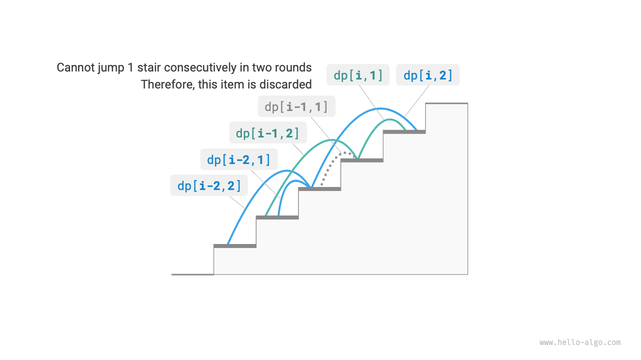
Figure 14-9 Recurrence relation considering constraints
Finally, return \(dp[n, 1] + dp[n, 2]\), where the sum of the two represents the total number of ways to climb to the \(n\)-th step:
def climbing_stairs_constraint_dp(n: int) -> int:
    """Climbing stairs with constraint: Dynamic programming"""
    if n == 1 or n == 2:
        return 1
    # Initialize dp table, used to store solutions to subproblems
    dp = [[0] * 3 for _ in range(n + 1)]
    # Initial state: preset the solution to the smallest subproblem
    dp[1][1], dp[1][2] = 1, 0
    dp[2][1], dp[2][2] = 0, 1
    # State transition: gradually solve larger subproblems from smaller ones
    for i in range(3, n + 1):
        dp[i][1] = dp[i - 1][2]
        dp[i][2] = dp[i - 2][1] + dp[i - 2][2]
    return dp[n][1] + dp[n][2]
/* Climbing stairs with constraint: Dynamic programming */
int climbingStairsConstraintDP(int n) {
    if (n == 1 || n == 2) {
        return 1;
    }
    // Initialize dp table, used to store solutions to subproblems
    vector<vector<int>> dp(n + 1, vector<int>(3, 0));
    // Initial state: preset the solution to the smallest subproblem
    dp[1][1] = 1;
    dp[1][2] = 0;
    dp[2][1] = 0;
    dp[2][2] = 1;
    // State transition: gradually solve larger subproblems from smaller ones
    for (int i = 3; i <= n; i++) {
        dp[i][1] = dp[i - 1][2];
        dp[i][2] = dp[i - 2][1] + dp[i - 2][2];
    }
    return dp[n][1] + dp[n][2];
}
/* Climbing stairs with constraint: Dynamic programming */
int climbingStairsConstraintDP(int n) {
    if (n == 1 || n == 2) {
        return 1;
    }
    // Initialize dp table, used to store solutions to subproblems
    int[][] dp = new int[n + 1][3];
    // Initial state: preset the solution to the smallest subproblem
    dp[1][1] = 1;
    dp[1][2] = 0;
    dp[2][1] = 0;
    dp[2][2] = 1;
    // State transition: gradually solve larger subproblems from smaller ones
    for (int i = 3; i <= n; i++) {
        dp[i][1] = dp[i - 1][2];
        dp[i][2] = dp[i - 2][1] + dp[i - 2][2];
    }
    return dp[n][1] + dp[n][2];
}
/* Climbing stairs with constraint: Dynamic programming */
int ClimbingStairsConstraintDP(int n) {
    if (n == 1 || n == 2) {
        return 1;
    }
    // Initialize dp table, used to store solutions to subproblems
    int[,] dp = new int[n + 1, 3];
    // Initial state: preset the solution to the smallest subproblem
    dp[1, 1] = 1;
    dp[1, 2] = 0;
    dp[2, 1] = 0;
    dp[2, 2] = 1;
    // State transition: gradually solve larger subproblems from smaller ones
    for (int i = 3; i <= n; i++) {
        dp[i, 1] = dp[i - 1, 2];
        dp[i, 2] = dp[i - 2, 1] + dp[i - 2, 2];
    }
    return dp[n, 1] + dp[n, 2];
}
/* Climbing stairs with constraint: Dynamic programming */
func climbingStairsConstraintDP(n int) int {
    if n == 1 || n == 2 {
        return 1
    }
    // Initialize dp table, used to store solutions to subproblems
    dp := make([][3]int, n+1)
    // Initial state: preset the solution to the smallest subproblem
    dp[1][1] = 1
    dp[1][2] = 0
    dp[2][1] = 0
    dp[2][2] = 1
    // State transition: gradually solve larger subproblems from smaller ones
    for i := 3; i <= n; i++ {
        dp[i][1] = dp[i-1][2]
        dp[i][2] = dp[i-2][1] + dp[i-2][2]
    }
    return dp[n][1] + dp[n][2]
}
/* Climbing stairs with constraint: Dynamic programming */
func climbingStairsConstraintDP(n: Int) -> Int {
    if n == 1 || n == 2 {
        return 1
    }
    // Initialize dp table, used to store solutions to subproblems
    var dp = Array(repeating: Array(repeating: 0, count: 3), count: n + 1)
    // Initial state: preset the solution to the smallest subproblem
    dp[1][1] = 1
    dp[1][2] = 0
    dp[2][1] = 0
    dp[2][2] = 1
    // State transition: gradually solve larger subproblems from smaller ones
    for i in 3 ... n {
        dp[i][1] = dp[i - 1][2]
        dp[i][2] = dp[i - 2][1] + dp[i - 2][2]
    }
    return dp[n][1] + dp[n][2]
}
/* Climbing stairs with constraint: Dynamic programming */
function climbingStairsConstraintDP(n) {
    if (n === 1 || n === 2) {
        return 1;
    }
    // Initialize dp table, used to store solutions to subproblems
    const dp = Array.from(new Array(n + 1), () => new Array(3));
    // Initial state: preset the solution to the smallest subproblem
    dp[1][1] = 1;
    dp[1][2] = 0;
    dp[2][1] = 0;
    dp[2][2] = 1;
    // State transition: gradually solve larger subproblems from smaller ones
    for (let i = 3; i <= n; i++) {
        dp[i][1] = dp[i - 1][2];
        dp[i][2] = dp[i - 2][1] + dp[i - 2][2];
    }
    return dp[n][1] + dp[n][2];
}
/* Climbing stairs with constraint: Dynamic programming */
function climbingStairsConstraintDP(n: number): number {
    if (n === 1 || n === 2) {
        return 1;
    }
    // Initialize dp table, used to store solutions to subproblems
    const dp = Array.from({ length: n + 1 }, () => new Array(3));
    // Initial state: preset the solution to the smallest subproblem
    dp[1][1] = 1;
    dp[1][2] = 0;
    dp[2][1] = 0;
    dp[2][2] = 1;
    // State transition: gradually solve larger subproblems from smaller ones
    for (let i = 3; i <= n; i++) {
        dp[i][1] = dp[i - 1][2];
        dp[i][2] = dp[i - 2][1] + dp[i - 2][2];
    }
    return dp[n][1] + dp[n][2];
}
/* Climbing stairs with constraint: Dynamic programming */
int climbingStairsConstraintDP(int n) {
  if (n == 1 || n == 2) {
    return 1;
  }
  // Initialize dp table, used to store solutions to subproblems
  List<List<int>> dp = List.generate(n + 1, (index) => List.filled(3, 0));
  // Initial state: preset the solution to the smallest subproblem
  dp[1][1] = 1;
  dp[1][2] = 0;
  dp[2][1] = 0;
  dp[2][2] = 1;
  // State transition: gradually solve larger subproblems from smaller ones
  for (int i = 3; i <= n; i++) {
    dp[i][1] = dp[i - 1][2];
    dp[i][2] = dp[i - 2][1] + dp[i - 2][2];
  }
  return dp[n][1] + dp[n][2];
}
/* Climbing stairs with constraint: Dynamic programming */
fn climbing_stairs_constraint_dp(n: usize) -> i32 {
    if n == 1 || n == 2 {
        return 1;
    };
    // Initialize dp table, used to store solutions to subproblems
    let mut dp = vec![vec![-1; 3]; n + 1];
    // Initial state: preset the solution to the smallest subproblem
    dp[1][1] = 1;
    dp[1][2] = 0;
    dp[2][1] = 0;
    dp[2][2] = 1;
    // State transition: gradually solve larger subproblems from smaller ones
    for i in 3..=n {
        dp[i][1] = dp[i - 1][2];
        dp[i][2] = dp[i - 2][1] + dp[i - 2][2];
    }
    dp[n][1] + dp[n][2]
}
/* Climbing stairs with constraint: Dynamic programming */
int climbingStairsConstraintDP(int n) {
    if (n == 1 || n == 2) {
        return 1;
    }
    // Initialize dp table, used to store solutions to subproblems
    int **dp = malloc((n + 1) * sizeof(int *));
    for (int i = 0; i <= n; i++) {
        dp[i] = calloc(3, sizeof(int));
    }
    // Initial state: preset the solution to the smallest subproblem
    dp[1][1] = 1;
    dp[1][2] = 0;
    dp[2][1] = 0;
    dp[2][2] = 1;
    // State transition: gradually solve larger subproblems from smaller ones
    for (int i = 3; i <= n; i++) {
        dp[i][1] = dp[i - 1][2];
        dp[i][2] = dp[i - 2][1] + dp[i - 2][2];
    }
    int res = dp[n][1] + dp[n][2];
    // Free memory
    for (int i = 0; i <= n; i++) {
        free(dp[i]);
    }
    free(dp);
    return res;
}
/* Climbing stairs with constraint: Dynamic programming */
fun climbingStairsConstraintDP(n: Int): Int {
    if (n == 1 || n == 2) {
        return 1
    }
    // Initialize dp table, used to store solutions to subproblems
    val dp = Array(n + 1) { IntArray(3) }
    // Initial state: preset the solution to the smallest subproblem
    dp[1][1] = 1
    dp[1][2] = 0
    dp[2][1] = 0
    dp[2][2] = 1
    // State transition: gradually solve larger subproblems from smaller ones
    for (i in 3..n) {
        dp[i][1] = dp[i - 1][2]
        dp[i][2] = dp[i - 2][1] + dp[i - 2][2]
    }
    return dp[n][1] + dp[n][2]
}
### Climbing stairs with constraint: DP ###
def climbing_stairs_constraint_dp(n)
  return 1 if n == 1 || n == 2

  # Initialize dp table, used to store solutions to subproblems
  dp = Array.new(n + 1) { Array.new(3, 0) }
  # Initial state: preset the solution to the smallest subproblem
  dp[1][1], dp[1][2] = 1, 0
  dp[2][1], dp[2][2] = 0, 1
  # State transition: gradually solve larger subproblems from smaller ones
  for i in 3...(n + 1)
    dp[i][1] = dp[i - 1][2]
    dp[i][2] = dp[i - 2][1] + dp[i - 2][2]
  end

  dp[n][1] + dp[n][2]
end
In the above case, since we only need to consider one more preceding state, we can still make the problem satisfy no aftereffects by expanding the state definition. However, some problems have very severe "aftereffects".
Climbing stairs with obstacle generation
Given a staircase with \(n\) steps, where you can climb \(1\) or \(2\) steps at a time. Whenever you reach the \(i\)-th step, the system automatically places an obstacle on the \(2i\)-th step, and no subsequent round is allowed to jump to the \(2i\)-th step. For example, if the first two rounds jump to the \(2\)nd and \(3\)rd steps, then afterwards you cannot jump to the \(4\)th and \(6\)th steps. How many ways are there to climb to the top?
In this problem, the next jump depends on all past states, because each jump places obstacles on higher steps, affecting future jumps. For such problems, dynamic programming is often difficult to solve.
In fact, many complex combinatorial optimization problems (such as the traveling salesman problem) do not satisfy no aftereffects. For such problems, we usually use other methods, such as heuristic search, genetic algorithms, and reinforcement learning, to obtain usable locally optimal solutions within a limited time.