2.2 Iteration and Recursion
In algorithms, repeatedly executing a task is very common and closely related to complexity analysis. Therefore, before introducing time complexity and space complexity, let's first understand how to implement repeated task execution in programs, namely the two basic program control structures: iteration and recursion.
2.2.1 Iteration
Iteration is a control structure for repeatedly executing a task. In iteration, a program repeatedly executes a segment of code under certain conditions until those conditions are no longer satisfied.
1. For Loop
The for loop is one of the most common forms of iteration, suitable for use when the number of iterations is known in advance.
The following function implements the summation \(1 + 2 + \dots + n\) using a for loop, with the result stored in the variable res. Note that in Python, range(a, b) corresponds to a "left-closed, right-open" interval, with the traversal range being \(a, a + 1, \dots, b-1\):
Figure 2-1 shows the flowchart of this summation function.
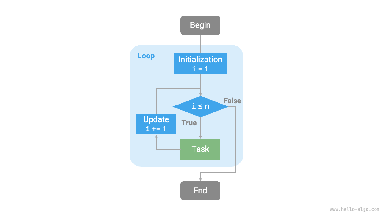
Figure 2-1 Flowchart of the summation function
The number of operations in this summation function is proportional to the input data size \(n\), or has a "linear relationship". In fact, time complexity describes precisely this "linear relationship". Related content will be introduced in detail in the next section.
2. While Loop
Similar to the for loop, the while loop is also a method for implementing iteration. In a while loop, the program first checks the condition in each round; if the condition is true, it continues execution, otherwise it ends the loop.
Below we use a while loop to implement the summation \(1 + 2 + \dots + n\):
The while loop has greater flexibility than the for loop. In a while loop, we can freely design the initialization and update steps of the condition variable.
For example, in the following code, the condition variable \(i\) is updated twice per round, which is not convenient to implement using a for loop:
Overall, for loops have more compact code, while while loops are more flexible; both can implement iterative structures. The choice of which to use should be determined based on the requirements of the specific problem.
3. Nested Loops
We can nest one loop structure inside another. Below is an example using for loops:
/* Nested for loop */
char *nestedForLoop(int n) {
    // n * n is the number of points, "(i, j), " string max length is 6+10*2, plus extra space for null character \0
    int size = n * n * 26 + 1;
    char *res = malloc(size * sizeof(char));
    // Loop i = 1, 2, ..., n-1, n
    for (int i = 1; i <= n; i++) {
        // Loop j = 1, 2, ..., n-1, n
        for (int j = 1; j <= n; j++) {
            char tmp[26];
            snprintf(tmp, sizeof(tmp), "(%d, %d), ", i, j);
            strncat(res, tmp, size - strlen(res) - 1);
        }
    }
    return res;
}
Figure 2-2 shows the flowchart of this nested loop.
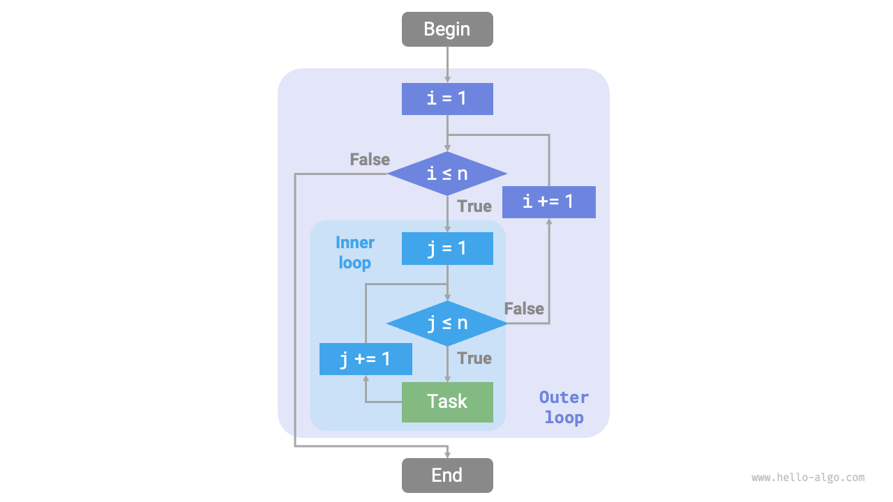
Figure 2-2 Flowchart of nested loops
In this case, the number of operations of the function is proportional to \(n^2\), or the algorithm's running time has a "quadratic relationship" with the input data size \(n\).
We can continue adding nested loops, where each additional level of nesting can be viewed as an increase in dimensionality, raising the time complexity to a "cubic relationship", a "quartic relationship", and so on.
2.2.2 Recursion
Recursion is an algorithmic strategy that solves problems by having a function call itself. It mainly consists of two phases.
- Descend: The program continuously calls itself deeper, usually passing in smaller or more simplified parameters, until reaching a "termination condition".
- Ascend: After triggering the "termination condition", the program returns layer by layer from the deepest recursive function, aggregating the result of each layer.
From an implementation perspective, recursive code mainly consists of three elements.
- Termination condition: Used to determine when to switch from "descending" to "ascending".
- Recursive call: Corresponds to "descending", where the function calls itself, usually with smaller or more simplified parameters.
- Return result: Corresponds to "ascending", returning the result of the current recursion level to the previous layer.
Observe the following code. We only need to call the function recur(n) to complete the calculation of \(1 + 2 + \dots + n\):
Figure 2-3 shows the recursive process of this function.
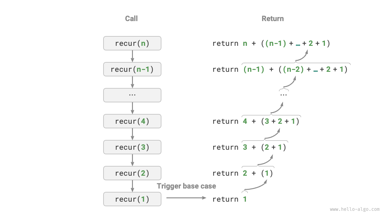
Figure 2-3 Recursive process of the summation function
Although from a computational perspective, iteration and recursion can achieve the same results, they represent two completely different paradigms for thinking about and solving problems.
- Iteration: Solves problems "bottom-up". Starting from the most basic steps, these steps are then repeatedly executed or accumulated until the task is complete.
- Recursion: Solves problems "top-down". The original problem is decomposed into smaller subproblems that have the same form as the original problem. These subproblems continue to be decomposed into even smaller subproblems until reaching the base case (where the solution is known).
Taking the above summation function as an example, let the problem be \(f(n) = 1 + 2 + \dots + n\).
- Iteration: Simulates the summation process in a loop, traversing from \(1\) to \(n\), performing the summation operation in each round to obtain \(f(n)\).
- Recursion: Decomposes the problem into the subproblem \(f(n) = n + f(n-1)\), continuously decomposing (recursively) until terminating at the base case \(f(1) = 1\).
1. Call Stack
Each time a recursive function calls itself, the system allocates memory for the newly invoked function to store local variables, call addresses, and other information. This leads to two consequences.
- The function's context data is stored in a memory area called "stack frame space", which is not released until the function returns. Therefore, recursion usually consumes more memory space than iteration.
- Recursive function calls incur additional overhead. Therefore, recursion is usually less time-efficient than loops.
As shown in Figure 2-4, before the termination condition is triggered, there are \(n\) unreturned recursive functions existing simultaneously, with a recursion depth of \(n\).
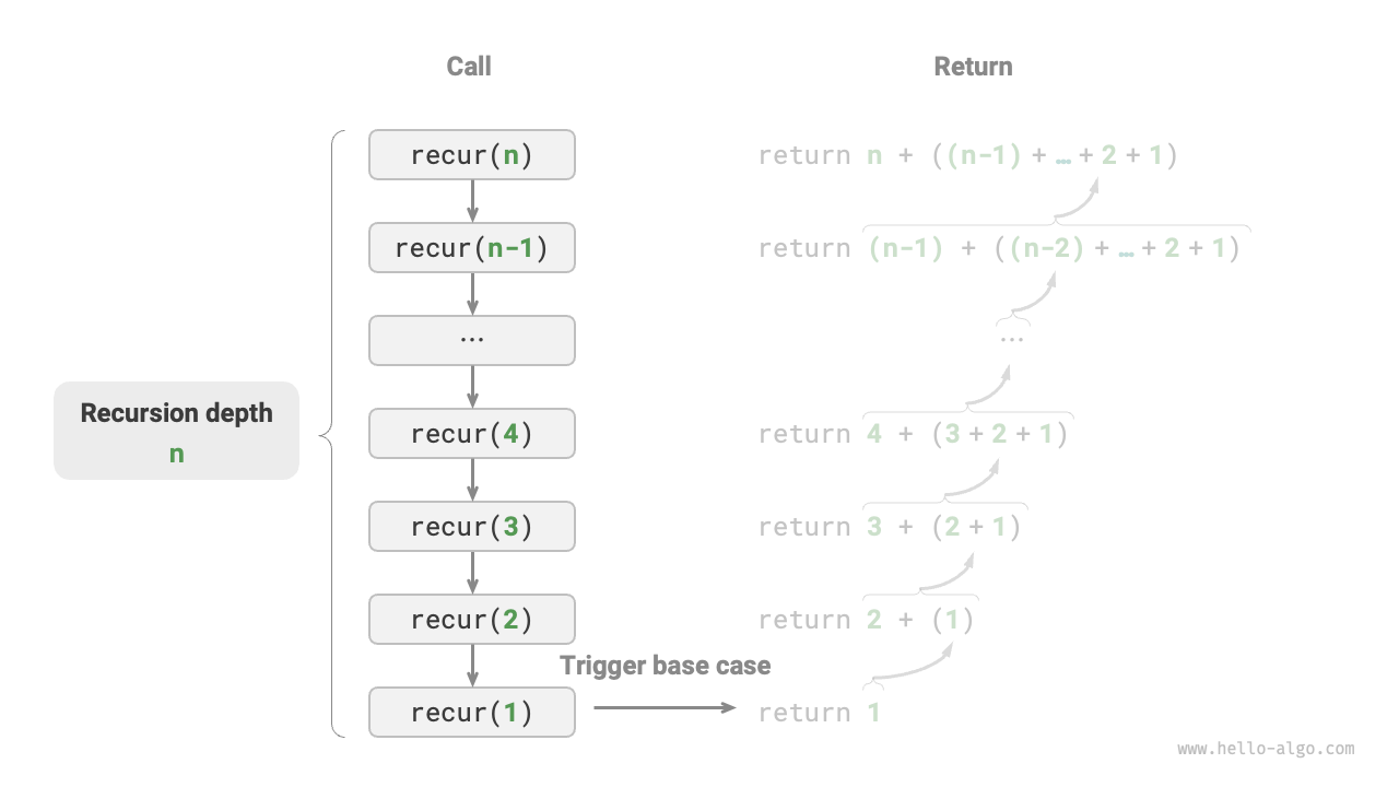
Figure 2-4 Recursion call depth
In practice, the recursion depth allowed by programming languages is usually limited, and excessively deep recursion may lead to stack overflow errors.
2. Tail Recursion
Interestingly, if a function makes the recursive call as the very last step before returning, the compiler or interpreter may optimize it so that its space efficiency is comparable to iteration. This case is called tail recursion.
- Regular recursion: When a function returns to the previous level, it needs to continue executing code, so the system needs to save the context of the previous layer's call.
- Tail recursion: The recursive call is the last operation before the function returns, meaning that after returning to the previous level, there is no need to continue executing other operations, so the system does not need to save the context of the previous layer's function.
Taking the calculation of \(1 + 2 + \dots + n\) as an example, we can set the result variable res as a function parameter to implement tail recursion:
The execution process of tail recursion is shown in Figure 2-5. Comparing regular recursion and tail recursion, the summation operation is performed at different points.
- Regular recursion: The summation operation is performed during the "ascending" process, requiring an additional summation operation after each layer returns.
- Tail recursion: The summation operation is performed during the "descending" process; the "ascending" process only needs to return layer by layer.
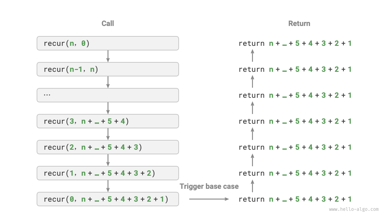
Figure 2-5 Tail recursion process
Tip
Please note that many compilers or interpreters do not support tail recursion optimization. For example, Python does not support tail recursion optimization by default, so even if a function is in tail recursive form, it may still encounter stack overflow issues.
3. Recursion Tree
When dealing with algorithmic problems related to "divide and conquer", recursion often provides a more intuitive approach and more readable code than iteration. Taking the "Fibonacci sequence" as an example.
Question
Given a Fibonacci sequence \(0, 1, 1, 2, 3, 5, 8, 13, \dots\), find the \(n\)-th number in the sequence.
Let the \(n\)-th number of the Fibonacci sequence be \(f(n)\). Two conclusions can be easily obtained.
- The first two numbers of the sequence are \(f(1) = 0\) and \(f(2) = 1\).
- Each number in the sequence is the sum of the previous two numbers, i.e., \(f(n) = f(n - 1) + f(n - 2)\).
Following the recurrence relation to make recursive calls, with the first two numbers as termination conditions, we can write the recursive code. Calling fib(n) will give us the \(n\)-th number of the Fibonacci sequence:
Observing the above code, we make two recursive calls within the function, meaning that one call produces two call branches. As shown in Figure 2-6, this repeated recursive calling eventually produces a recursion tree with \(n\) levels.
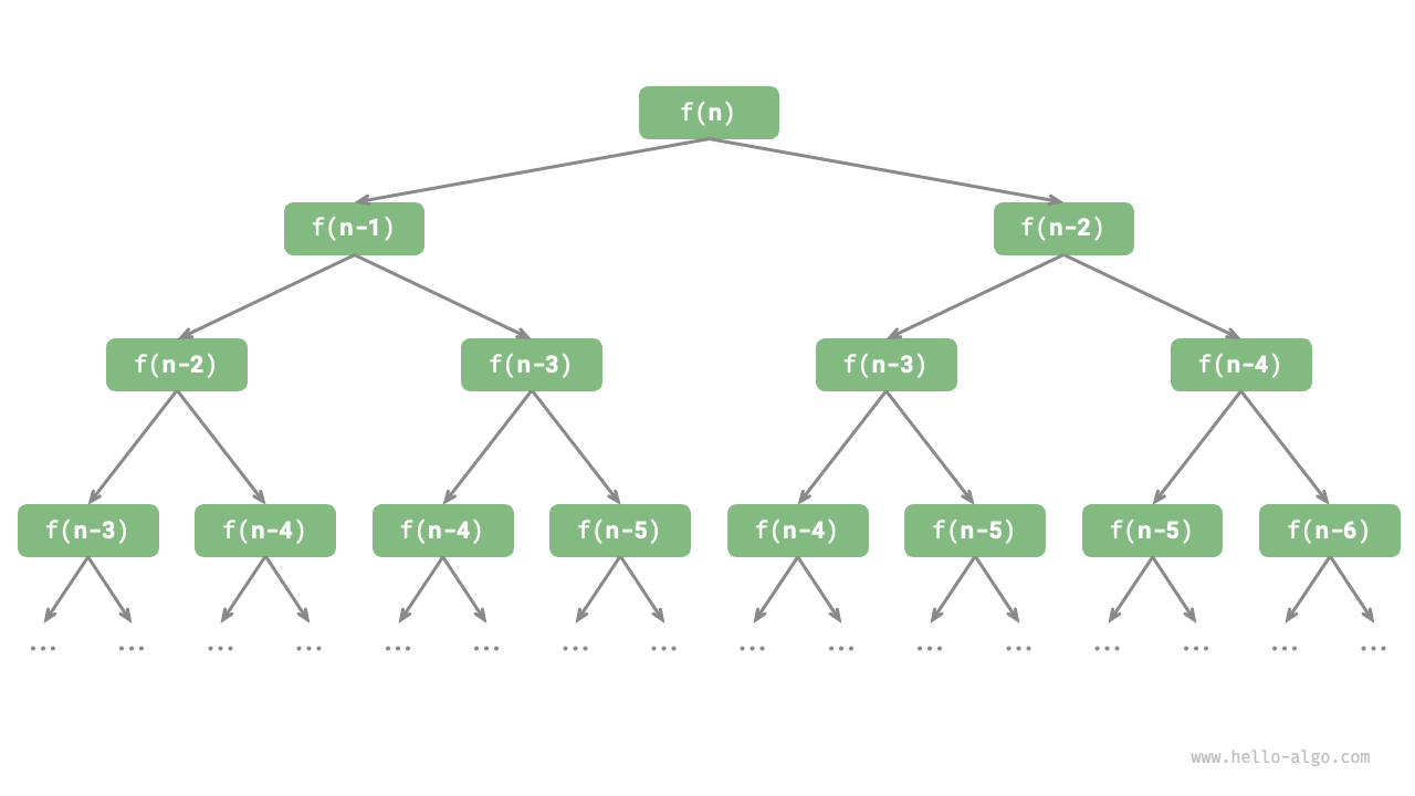
Figure 2-6 Recursion tree of the Fibonacci sequence
Fundamentally, recursion embodies the paradigm of "decomposing a problem into smaller subproblems", and this divide-and-conquer strategy is crucial.
- From an algorithmic perspective, many important algorithmic strategies such as searching, sorting, backtracking, divide and conquer, and dynamic programming directly or indirectly apply this way of thinking.
- From a data structure perspective, recursion is naturally suited for handling problems related to linked lists, trees, and graphs, because they are well-suited for analysis using divide-and-conquer thinking.
2.2.3 Comparison of the Two
Summarizing the above content, as shown in Table 2-1, iteration and recursion differ in implementation, performance, and applicability.
Table 2-1 Comparison of iteration and recursion characteristics
| Iteration | Recursion | |
|---|---|---|
| Implementation | Loop structure | Function calls itself |
| Time efficiency | Generally more efficient, no function call overhead | Each function call incurs overhead |
| Memory usage | Usually uses a fixed amount of memory space | Accumulated function calls may use a large amount of stack frame space |
| Suitable problems | Suitable for simple loop tasks, with intuitive and readable code | Suitable for subproblem decomposition, such as trees, graphs, divide and conquer, backtracking, etc., with concise and clear code structure |
Tip
If you find the following content difficult to understand, you can review it after reading the "Stack" chapter.
What is the intrinsic relationship between iteration and recursion? Taking the above recursive function as an example, the summation operation is performed during the "ascending" phase of recursion. This means that the function called first actually completes its summation operation last, and this working mechanism is similar to the "last-in, first-out" principle of stacks.
In fact, recursive terminology such as "call stack" and "stack frame space" already hints at the close relationship between recursion and stacks.
- Descend: When a function is called, the system allocates a new stack frame on the "call stack" for that function to store the function's local variables, parameters, return address, and other data.
- Ascend: When the function completes execution and returns, the corresponding stack frame is removed from the "call stack", restoring the execution environment of the previous function.
Therefore, we can use an explicit stack to simulate the behavior of the call stack, thus transforming recursion into iterative form:
def for_loop_recur(n: int) -> int:
    """Simulate recursion using iteration"""
    # Use an explicit stack to simulate the system call stack
    stack = []
    res = 0
    # Recurse: recursive call
    for i in range(n, 0, -1):
        # Simulate "recurse" with "push"
        stack.append(i)
    # Return: return result
    while stack:
        # Simulate "return" with "pop"
        res += stack.pop()
    # res = 1+2+3+...+n
    return res
/* Simulate recursion using iteration */
int forLoopRecur(int n) {
    // Use an explicit stack to simulate the system call stack
    stack<int> stack;
    int res = 0;
    // Recurse: recursive call
    for (int i = n; i > 0; i--) {
        // Simulate "recurse" with "push"
        stack.push(i);
    }
    // Return: return result
    while (!stack.empty()) {
        // Simulate "return" with "pop"
        res += stack.top();
        stack.pop();
    }
    // res = 1+2+3+...+n
    return res;
}
/* Simulate recursion using iteration */
int forLoopRecur(int n) {
    // Use an explicit stack to simulate the system call stack
    Stack<Integer> stack = new Stack<>();
    int res = 0;
    // Recurse: recursive call
    for (int i = n; i > 0; i--) {
        // Simulate "recurse" with "push"
        stack.push(i);
    }
    // Return: return result
    while (!stack.isEmpty()) {
        // Simulate "return" with "pop"
        res += stack.pop();
    }
    // res = 1+2+3+...+n
    return res;
}
/* Simulate recursion using iteration */
int ForLoopRecur(int n) {
    // Use an explicit stack to simulate the system call stack
    Stack<int> stack = new();
    int res = 0;
    // Recurse: recursive call
    for (int i = n; i > 0; i--) {
        // Simulate "recurse" with "push"
        stack.Push(i);
    }
    // Return: return result
    while (stack.Count > 0) {
        // Simulate "return" with "pop"
        res += stack.Pop();
    }
    // res = 1+2+3+...+n
    return res;
}
/* Simulate recursion using iteration */
func forLoopRecur(n int) int {
    // Use an explicit stack to simulate the system call stack
    stack := list.New()
    res := 0
    // Recurse: recursive call
    for i := n; i > 0; i-- {
        // Simulate "recurse" with "push"
        stack.PushBack(i)
    }
    // Return: return result
    for stack.Len() != 0 {
        // Simulate "return" with "pop"
        res += stack.Back().Value.(int)
        stack.Remove(stack.Back())
    }
    // res = 1+2+3+...+n
    return res
}
/* Simulate recursion using iteration */
func forLoopRecur(n: Int) -> Int {
    // Use an explicit stack to simulate the system call stack
    var stack: [Int] = []
    var res = 0
    // Recurse: recursive call
    for i in (1 ... n).reversed() {
        // Simulate "recurse" with "push"
        stack.append(i)
    }
    // Return: return result
    while !stack.isEmpty {
        // Simulate "return" with "pop"
        res += stack.removeLast()
    }
    // res = 1+2+3+...+n
    return res
}
/* Simulate recursion using iteration */
function forLoopRecur(n) {
    // Use an explicit stack to simulate the system call stack
    const stack = [];
    let res = 0;
    // Recurse: recursive call
    for (let i = n; i > 0; i--) {
        // Simulate "recurse" with "push"
        stack.push(i);
    }
    // Return: return result
    while (stack.length) {
        // Simulate "return" with "pop"
        res += stack.pop();
    }
    // res = 1+2+3+...+n
    return res;
}
/* Simulate recursion using iteration */
function forLoopRecur(n: number): number {
    // Use an explicit stack to simulate the system call stack
    const stack: number[] = [];
    let res: number = 0;
    // Recurse: recursive call
    for (let i = n; i > 0; i--) {
        // Simulate "recurse" with "push"
        stack.push(i);
    }
    // Return: return result
    while (stack.length) {
        // Simulate "return" with "pop"
        res += stack.pop();
    }
    // res = 1+2+3+...+n
    return res;
}
/* Simulate recursion using iteration */
int forLoopRecur(int n) {
  // Use an explicit stack to simulate the system call stack
  List<int> stack = [];
  int res = 0;
  // Recurse: recursive call
  for (int i = n; i > 0; i--) {
    // Simulate "recurse" with "push"
    stack.add(i);
  }
  // Return: return result
  while (!stack.isEmpty) {
    // Simulate "return" with "pop"
    res += stack.removeLast();
  }
  // res = 1+2+3+...+n
  return res;
}
/* Simulate recursion using iteration */
fn for_loop_recur(n: i32) -> i32 {
    // Use an explicit stack to simulate the system call stack
    let mut stack = Vec::new();
    let mut res = 0;
    // Recurse: recursive call
    for i in (1..=n).rev() {
        // Simulate "recurse" with "push"
        stack.push(i);
    }
    // Return: return result
    while !stack.is_empty() {
        // Simulate "return" with "pop"
        res += stack.pop().unwrap();
    }
    // res = 1+2+3+...+n
    res
}
/* Simulate recursion using iteration */
int forLoopRecur(int n) {
    int stack[1000]; // Use a large array to simulate stack
    int top = -1;    // Stack top index
    int res = 0;
    // Recurse: recursive call
    for (int i = n; i > 0; i--) {
        // Simulate "recurse" with "push"
        stack[1 + top++] = i;
    }
    // Return: return result
    while (top >= 0) {
        // Simulate "return" with "pop"
        res += stack[top--];
    }
    // res = 1+2+3+...+n
    return res;
}
/* Simulate recursion using iteration */
fun forLoopRecur(n: Int): Int {
    // Use an explicit stack to simulate the system call stack
    val stack = Stack<Int>()
    var res = 0
    // Descend: recursive call
    for (i in n downTo 0) {
        // Simulate "recurse" with "push"
        stack.push(i)
    }
    // Return: return result
    while (stack.isNotEmpty()) {
        // Simulate "return" with "pop"
        res += stack.pop()
    }
    // res = 1+2+3+...+n
    return res
}
### Use iteration to simulate recursion ###
def for_loop_recur(n)
  # Use an explicit stack to simulate the system call stack
  stack = []
  res = 0

  # Recurse: recursive call
  for i in n.downto(0)
    # Simulate "recurse" with "push"
    stack << i
  end
  # Return: return result
  while !stack.empty?
    res += stack.pop
  end

  # res = 1+2+3+...+n
  res
end
Observing the above code, when recursion is transformed into iteration, the code becomes more complex. Although iteration and recursion can be converted into each other in many cases, it may not be worthwhile to do so for the following two reasons.
- The transformed code may be more difficult to understand and less readable.
- For some complex problems, simulating the behavior of the system call stack can be very difficult.
In summary, choosing between iteration and recursion depends on the nature of the specific problem. In programming practice, it is crucial to weigh the pros and cons of both and choose the appropriate method based on the context.