14.3 Dynamic Programming Problem-Solving Approach
The previous two sections introduced the main characteristics of dynamic programming problems. Next, let us explore two more practical issues together.
- How to determine whether a problem is a dynamic programming problem?
- What is the complete process for solving a dynamic programming problem, and where should we start?
14.3.1 Problem Identification
Generally speaking, if a problem contains overlapping subproblems, optimal substructure, and satisfies no aftereffects, then it is usually suitable for solving with dynamic programming. However, it is difficult to directly extract these characteristics from the problem description. Therefore, we usually relax the conditions and first observe whether the problem is suitable for solving with backtracking (exhaustive search).
Problems suitable for solving with backtracking usually satisfy the "decision tree model", which means the problem can be described using a tree structure, where each node represents a decision and each path represents a sequence of decisions.
In other words, if a problem contains an explicit concept of decisions, and the solution is generated through a series of decisions, then it satisfies the decision tree model and can usually be solved using backtracking.
On this basis, dynamic programming problems also have some positive indicators.
- The problem contains descriptions such as maximum (minimum) or most (least), indicating optimization.
- The problem's state can be represented using a list, multi-dimensional matrix, or tree, and a state has a recurrence relation with its surrounding states.
Correspondingly, there are also some negative indicators.
- The goal of the problem is to find all possible solutions, rather than finding the optimal solution.
- The problem description has obvious permutation and combination characteristics, requiring the return of specific multiple solutions.
If a problem satisfies the decision tree model and has relatively obvious positive indicators, we can assume it is a dynamic programming problem and verify that assumption during the solving process.
14.3.2 Problem-Solving Steps
The problem-solving process for dynamic programming varies depending on the nature and difficulty of the problem, but generally follows these steps: describe decisions, define states, establish the \(dp\) table, derive state transition equations, determine boundary conditions, etc.
To illustrate the problem-solving steps more vividly, we use a classic problem "minimum path sum" as an example.
Question
Given an \(n \times m\) two-dimensional grid grid in which each cell contains a non-negative integer representing its cost, a robot starts from the top-left cell and can only move down or right at each step until reaching the bottom-right cell. Return the minimum path sum from the top-left to the bottom-right.
Figure 14-10 shows an example where the minimum path sum for the given grid is \(13\).

Figure 14-10 Minimum path sum example data
Step 1: Think about the decisions in each round, define the state, and thus obtain the \(dp\) table
The decision in each round of this problem is to move one step down or right from the current cell. Let the row and column indices of the current cell be \([i, j]\). After moving down or right, the indices become \([i+1, j]\) or \([i, j+1]\). Therefore, the state should include two variables, the row index and column index, denoted as \([i, j]\).
State \([i, j]\) corresponds to the subproblem: the minimum path sum from the starting point \([0, 0]\) to \([i, j]\), denoted as \(dp[i, j]\).
From this, we obtain the two-dimensional \(dp\) matrix shown in Figure 14-11, whose size is the same as the input grid \(grid\).
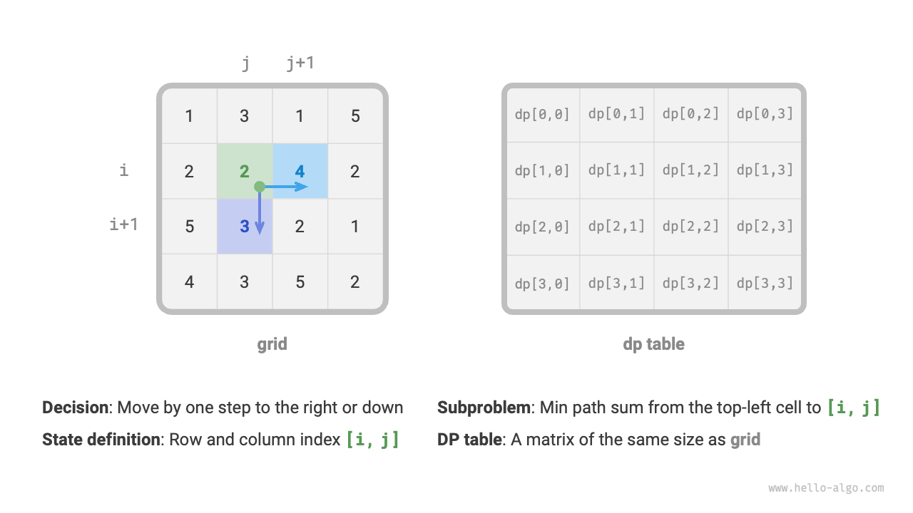
Figure 14-11 State definition and dp table
Note
The dynamic programming and backtracking processes can be described as a sequence of decisions, and the state consists of all decision variables. It should contain all variables describing the progress of problem-solving, and should contain sufficient information to derive the next state.
Each state corresponds to a subproblem, and we define a \(dp\) table to store the solutions to all subproblems. Each independent variable of the state is a dimension of the \(dp\) table. Essentially, the \(dp\) table is a mapping between states and solutions to subproblems.
Step 2: Identify the optimal substructure, and then derive the state transition equation
For state \([i, j]\), it can only transition from the cell above \([i-1, j]\) or the cell to the left \([i, j-1]\). Therefore, the optimal substructure is: the minimum path sum to reach \([i, j]\) is determined by the smaller of the minimum path sums of \([i, j-1]\) and \([i-1, j]\).
Based on the above analysis, the state transition equation shown in Figure 14-12 can be derived:
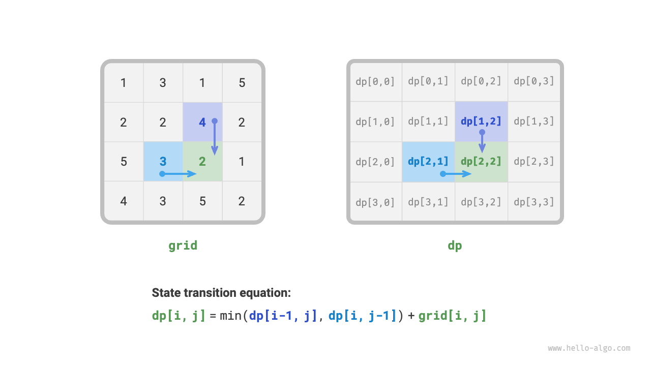
Figure 14-12 Optimal substructure and state transition equation
Note
Based on the defined \(dp\) table, think about the relationship between the original problem and subproblems, and find the method to construct the optimal solution to the original problem from the optimal solutions to the subproblems, which is the optimal substructure.
Once we identify the optimal substructure, we can use it to construct the state transition equation.
Step 3: Determine boundary conditions and state transition order
In this problem, states in the first row can only come from the state to their left, and states in the first column can only come from the state above them. Therefore, the first row \(i = 0\) and first column \(j = 0\) are boundary conditions.
As shown in Figure 14-13, since each cell transitions from the cell to its left and the cell above it, we use loops to traverse the matrix, with the outer loop traversing rows and the inner loop traversing columns.

Figure 14-13 Boundary conditions and state transition order
Note
Boundary conditions in dynamic programming are used to initialize the \(dp\) table, while in search they are used for pruning.
The core of state transition order is to ensure that when computing the solution to the current problem, all the smaller subproblems it depends on have already been computed correctly.
Based on the above analysis, we can directly write the dynamic programming code. However, subproblem decomposition is a top-down approach, so implementing in the order "brute force search \(\rightarrow\) memoization \(\rightarrow\) dynamic programming" is more aligned with thinking habits.
1. Method 1: Brute Force Search
Starting from state \([i, j]\), we continuously decompose it into smaller states \([i-1, j]\) and \([i, j-1]\). The recursive function includes the following elements.
- Recursive parameters: state \([i, j]\).
- Return value: minimum path sum from \([0, 0]\) to \([i, j]\), which is \(dp[i, j]\).
- Termination condition: when \(i = 0\) and \(j = 0\), return cost \(grid[0, 0]\).
- Pruning: when \(i < 0\) or \(j < 0\), the index is out of bounds, return cost \(+\infty\), representing infeasibility.
The implementation code is as follows:
def min_path_sum_dfs(grid: list[list[int]], i: int, j: int) -> int:
    """Minimum path sum: Brute-force search"""
    # If it's the top-left cell, terminate the search
    if i == 0 and j == 0:
        return grid[0][0]
    # If row or column index is out of bounds, return +∞ cost
    if i < 0 or j < 0:
        return inf
    # Calculate the minimum path cost from top-left to (i-1, j) and (i, j-1)
    up = min_path_sum_dfs(grid, i - 1, j)
    left = min_path_sum_dfs(grid, i, j - 1)
    # Return the minimum path cost from top-left to (i, j)
    return min(left, up) + grid[i][j]
/* Minimum path sum: Brute-force search */
int minPathSumDFS(vector<vector<int>> &grid, int i, int j) {
    // If it's the top-left cell, terminate the search
    if (i == 0 && j == 0) {
        return grid[0][0];
    }
    // If row or column index is out of bounds, return +∞ cost
    if (i < 0 || j < 0) {
        return INT_MAX;
    }
    // Calculate the minimum path cost from top-left to (i-1, j) and (i, j-1)
    int up = minPathSumDFS(grid, i - 1, j);
    int left = minPathSumDFS(grid, i, j - 1);
    // Return the minimum path cost from top-left to (i, j)
    return min(left, up) != INT_MAX ? min(left, up) + grid[i][j] : INT_MAX;
}
/* Minimum path sum: Brute-force search */
int minPathSumDFS(int[][] grid, int i, int j) {
    // If it's the top-left cell, terminate the search
    if (i == 0 && j == 0) {
        return grid[0][0];
    }
    // If row or column index is out of bounds, return +∞ cost
    if (i < 0 || j < 0) {
        return Integer.MAX_VALUE;
    }
    // Calculate the minimum path cost from top-left to (i-1, j) and (i, j-1)
    int up = minPathSumDFS(grid, i - 1, j);
    int left = minPathSumDFS(grid, i, j - 1);
    // Return the minimum path cost from top-left to (i, j)
    return Math.min(left, up) + grid[i][j];
}
/* Minimum path sum: Brute-force search */
int MinPathSumDFS(int[][] grid, int i, int j) {
    // If it's the top-left cell, terminate the search
    if (i == 0 && j == 0) {
        return grid[0][0];
    }
    // If row or column index is out of bounds, return +∞ cost
    if (i < 0 || j < 0) {
        return int.MaxValue;
    }
    // Calculate the minimum path cost from top-left to (i-1, j) and (i, j-1)
    int up = MinPathSumDFS(grid, i - 1, j);
    int left = MinPathSumDFS(grid, i, j - 1);
    // Return the minimum path cost from top-left to (i, j)
    return Math.Min(left, up) + grid[i][j];
}
/* Minimum path sum: Brute-force search */
func minPathSumDFS(grid [][]int, i, j int) int {
    // If it's the top-left cell, terminate the search
    if i == 0 && j == 0 {
        return grid[0][0]
    }
    // If row or column index is out of bounds, return +∞ cost
    if i < 0 || j < 0 {
        return math.MaxInt
    }
    // Calculate the minimum path cost from top-left to (i-1, j) and (i, j-1)
    up := minPathSumDFS(grid, i-1, j)
    left := minPathSumDFS(grid, i, j-1)
    // Return the minimum path cost from top-left to (i, j)
    return int(math.Min(float64(left), float64(up))) + grid[i][j]
}
/* Minimum path sum: Brute-force search */
func minPathSumDFS(grid: [[Int]], i: Int, j: Int) -> Int {
    // If it's the top-left cell, terminate the search
    if i == 0, j == 0 {
        return grid[0][0]
    }
    // If row or column index is out of bounds, return +∞ cost
    if i < 0 || j < 0 {
        return .max
    }
    // Calculate the minimum path cost from top-left to (i-1, j) and (i, j-1)
    let up = minPathSumDFS(grid: grid, i: i - 1, j: j)
    let left = minPathSumDFS(grid: grid, i: i, j: j - 1)
    // Return the minimum path cost from top-left to (i, j)
    return min(left, up) + grid[i][j]
}
/* Minimum path sum: Brute-force search */
function minPathSumDFS(grid, i, j) {
    // If it's the top-left cell, terminate the search
    if (i === 0 && j === 0) {
        return grid[0][0];
    }
    // If row or column index is out of bounds, return +∞ cost
    if (i < 0 || j < 0) {
        return Infinity;
    }
    // Calculate the minimum path cost from top-left to (i-1, j) and (i, j-1)
    const up = minPathSumDFS(grid, i - 1, j);
    const left = minPathSumDFS(grid, i, j - 1);
    // Return the minimum path cost from top-left to (i, j)
    return Math.min(left, up) + grid[i][j];
}
/* Minimum path sum: Brute-force search */
function minPathSumDFS(
    grid: Array<Array<number>>,
    i: number,
    j: number
): number {
    // If it's the top-left cell, terminate the search
    if (i === 0 && j == 0) {
        return grid[0][0];
    }
    // If row or column index is out of bounds, return +∞ cost
    if (i < 0 || j < 0) {
        return Infinity;
    }
    // Calculate the minimum path cost from top-left to (i-1, j) and (i, j-1)
    const up = minPathSumDFS(grid, i - 1, j);
    const left = minPathSumDFS(grid, i, j - 1);
    // Return the minimum path cost from top-left to (i, j)
    return Math.min(left, up) + grid[i][j];
}
/* Minimum path sum: Brute-force search */
int minPathSumDFS(List<List<int>> grid, int i, int j) {
  // If it's the top-left cell, terminate the search
  if (i == 0 && j == 0) {
    return grid[0][0];
  }
  // If row or column index is out of bounds, return +∞ cost
  if (i < 0 || j < 0) {
    // In Dart, int type is fixed-range integer, no value representing "infinity"
    return BigInt.from(2).pow(31).toInt();
  }
  // Calculate the minimum path cost from top-left to (i-1, j) and (i, j-1)
  int up = minPathSumDFS(grid, i - 1, j);
  int left = minPathSumDFS(grid, i, j - 1);
  // Return the minimum path cost from top-left to (i, j)
  return min(left, up) + grid[i][j];
}
/* Minimum path sum: Brute-force search */
fn min_path_sum_dfs(grid: &Vec<Vec<i32>>, i: i32, j: i32) -> i32 {
    // If it's the top-left cell, terminate the search
    if i == 0 && j == 0 {
        return grid[0][0];
    }
    // If row or column index is out of bounds, return +∞ cost
    if i < 0 || j < 0 {
        return i32::MAX;
    }
    // Calculate the minimum path cost from top-left to (i-1, j) and (i, j-1)
    let up = min_path_sum_dfs(grid, i - 1, j);
    let left = min_path_sum_dfs(grid, i, j - 1);
    // Return the minimum path cost from top-left to (i, j)
    std::cmp::min(left, up) + grid[i as usize][j as usize]
}
/* Minimum path sum: Brute-force search */
int minPathSumDFS(int grid[MAX_SIZE][MAX_SIZE], int i, int j) {
    // If it's the top-left cell, terminate the search
    if (i == 0 && j == 0) {
        return grid[0][0];
    }
    // If row or column index is out of bounds, return +∞ cost
    if (i < 0 || j < 0) {
        return INT_MAX;
    }
    // Calculate the minimum path cost from top-left to (i-1, j) and (i, j-1)
    int up = minPathSumDFS(grid, i - 1, j);
    int left = minPathSumDFS(grid, i, j - 1);
    // Return the minimum path cost from top-left to (i, j)
    return myMin(left, up) != INT_MAX ? myMin(left, up) + grid[i][j] : INT_MAX;
}
/* Minimum path sum: Brute-force search */
fun minPathSumDFS(grid: Array<IntArray>, i: Int, j: Int): Int {
    // If it's the top-left cell, terminate the search
    if (i == 0 && j == 0) {
        return grid[0][0]
    }
    // If row or column index is out of bounds, return +∞ cost
    if (i < 0 || j < 0) {
        return Int.MAX_VALUE
    }
    // Calculate the minimum path cost from top-left to (i-1, j) and (i, j-1)
    val up = minPathSumDFS(grid, i - 1, j)
    val left = minPathSumDFS(grid, i, j - 1)
    // Return the minimum path cost from top-left to (i, j)
    return min(left, up) + grid[i][j]
}
### Minimum path sum: brute force search ###
def min_path_sum_dfs(grid, i, j)
  # If it's the top-left cell, terminate the search
  return grid[i][j] if i == 0 && j == 0
  # If row or column index is out of bounds, return +∞ cost
  return Float::INFINITY if i < 0 || j < 0
  # Calculate the minimum path cost from top-left to (i-1, j) and (i, j-1)
  up = min_path_sum_dfs(grid, i - 1, j)
  left = min_path_sum_dfs(grid, i, j - 1)
  # Return the minimum path cost from top-left to (i, j)
  [left, up].min + grid[i][j]
end
Figure 14-14 shows the recursion tree rooted at \(dp[2, 1]\), which includes some overlapping subproblems whose number will increase sharply as the size of grid grid grows.
Essentially, the reason for overlapping subproblems is: there are multiple paths from the top-left corner to reach a certain cell.
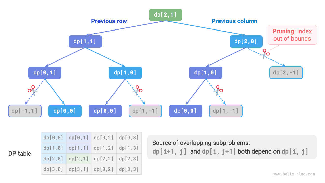
Figure 14-14 Brute force search recursion tree
Each state has two choices, down and right, so the total number of steps from the top-left corner to the bottom-right corner is \(m + n - 2\), giving a worst-case time complexity of \(O(2^{m + n})\), where \(n\) and \(m\) are the number of rows and columns of the grid, respectively. Note that this calculation does not account for situations near the grid boundaries, where only one choice remains when reaching the grid boundary, so the actual number of paths will be somewhat less.
2. Method 2: Memoization
We introduce a memo list mem of the same size as grid grid to record the solutions to subproblems and prune overlapping subproblems:
def min_path_sum_dfs_mem(
    grid: list[list[int]], mem: list[list[int]], i: int, j: int
) -> int:
    """Minimum path sum: Memoization search"""
    # If it's the top-left cell, terminate the search
    if i == 0 and j == 0:
        return grid[0][0]
    # If row or column index is out of bounds, return +∞ cost
    if i < 0 or j < 0:
        return inf
    # If there's a record, return it directly
    if mem[i][j] != -1:
        return mem[i][j]
    # Minimum path cost for left and upper cells
    up = min_path_sum_dfs_mem(grid, mem, i - 1, j)
    left = min_path_sum_dfs_mem(grid, mem, i, j - 1)
    # Record and return the minimum path cost from top-left to (i, j)
    mem[i][j] = min(left, up) + grid[i][j]
    return mem[i][j]
/* Minimum path sum: Memoization search */
int minPathSumDFSMem(vector<vector<int>> &grid, vector<vector<int>> &mem, int i, int j) {
    // If it's the top-left cell, terminate the search
    if (i == 0 && j == 0) {
        return grid[0][0];
    }
    // If row or column index is out of bounds, return +∞ cost
    if (i < 0 || j < 0) {
        return INT_MAX;
    }
    // If there's a record, return it directly
    if (mem[i][j] != -1) {
        return mem[i][j];
    }
    // Minimum path cost for left and upper cells
    int up = minPathSumDFSMem(grid, mem, i - 1, j);
    int left = minPathSumDFSMem(grid, mem, i, j - 1);
    // Record and return the minimum path cost from top-left to (i, j)
    mem[i][j] = min(left, up) != INT_MAX ? min(left, up) + grid[i][j] : INT_MAX;
    return mem[i][j];
}
/* Minimum path sum: Memoization search */
int minPathSumDFSMem(int[][] grid, int[][] mem, int i, int j) {
    // If it's the top-left cell, terminate the search
    if (i == 0 && j == 0) {
        return grid[0][0];
    }
    // If row or column index is out of bounds, return +∞ cost
    if (i < 0 || j < 0) {
        return Integer.MAX_VALUE;
    }
    // If there's a record, return it directly
    if (mem[i][j] != -1) {
        return mem[i][j];
    }
    // Minimum path cost for left and upper cells
    int up = minPathSumDFSMem(grid, mem, i - 1, j);
    int left = minPathSumDFSMem(grid, mem, i, j - 1);
    // Record and return the minimum path cost from top-left to (i, j)
    mem[i][j] = Math.min(left, up) + grid[i][j];
    return mem[i][j];
}
/* Minimum path sum: Memoization search */
int MinPathSumDFSMem(int[][] grid, int[][] mem, int i, int j) {
    // If it's the top-left cell, terminate the search
    if (i == 0 && j == 0) {
        return grid[0][0];
    }
    // If row or column index is out of bounds, return +∞ cost
    if (i < 0 || j < 0) {
        return int.MaxValue;
    }
    // If there's a record, return it directly
    if (mem[i][j] != -1) {
        return mem[i][j];
    }
    // Minimum path cost for left and upper cells
    int up = MinPathSumDFSMem(grid, mem, i - 1, j);
    int left = MinPathSumDFSMem(grid, mem, i, j - 1);
    // Record and return the minimum path cost from top-left to (i, j)
    mem[i][j] = Math.Min(left, up) + grid[i][j];
    return mem[i][j];
}
/* Minimum path sum: Memoization search */
func minPathSumDFSMem(grid, mem [][]int, i, j int) int {
    // If it's the top-left cell, terminate the search
    if i == 0 && j == 0 {
        return grid[0][0]
    }
    // If row or column index is out of bounds, return +∞ cost
    if i < 0 || j < 0 {
        return math.MaxInt
    }
    // If there's a record, return it directly
    if mem[i][j] != -1 {
        return mem[i][j]
    }
    // Minimum path cost for left and upper cells
    up := minPathSumDFSMem(grid, mem, i-1, j)
    left := minPathSumDFSMem(grid, mem, i, j-1)
    // Record and return the minimum path cost from top-left to (i, j)
    mem[i][j] = int(math.Min(float64(left), float64(up))) + grid[i][j]
    return mem[i][j]
}
/* Minimum path sum: Memoization search */
func minPathSumDFSMem(grid: [[Int]], mem: inout [[Int]], i: Int, j: Int) -> Int {
    // If it's the top-left cell, terminate the search
    if i == 0, j == 0 {
        return grid[0][0]
    }
    // If row or column index is out of bounds, return +∞ cost
    if i < 0 || j < 0 {
        return .max
    }
    // If there's a record, return it directly
    if mem[i][j] != -1 {
        return mem[i][j]
    }
    // Minimum path cost for left and upper cells
    let up = minPathSumDFSMem(grid: grid, mem: &mem, i: i - 1, j: j)
    let left = minPathSumDFSMem(grid: grid, mem: &mem, i: i, j: j - 1)
    // Record and return the minimum path cost from top-left to (i, j)
    mem[i][j] = min(left, up) + grid[i][j]
    return mem[i][j]
}
/* Minimum path sum: Memoization search */
function minPathSumDFSMem(grid, mem, i, j) {
    // If it's the top-left cell, terminate the search
    if (i === 0 && j === 0) {
        return grid[0][0];
    }
    // If row or column index is out of bounds, return +∞ cost
    if (i < 0 || j < 0) {
        return Infinity;
    }
    // If there's a record, return it directly
    if (mem[i][j] !== -1) {
        return mem[i][j];
    }
    // Minimum path cost for left and upper cells
    const up = minPathSumDFSMem(grid, mem, i - 1, j);
    const left = minPathSumDFSMem(grid, mem, i, j - 1);
    // Record and return the minimum path cost from top-left to (i, j)
    mem[i][j] = Math.min(left, up) + grid[i][j];
    return mem[i][j];
}
/* Minimum path sum: Memoization search */
function minPathSumDFSMem(
    grid: Array<Array<number>>,
    mem: Array<Array<number>>,
    i: number,
    j: number
): number {
    // If it's the top-left cell, terminate the search
    if (i === 0 && j === 0) {
        return grid[0][0];
    }
    // If row or column index is out of bounds, return +∞ cost
    if (i < 0 || j < 0) {
        return Infinity;
    }
    // If there's a record, return it directly
    if (mem[i][j] != -1) {
        return mem[i][j];
    }
    // Minimum path cost for left and upper cells
    const up = minPathSumDFSMem(grid, mem, i - 1, j);
    const left = minPathSumDFSMem(grid, mem, i, j - 1);
    // Record and return the minimum path cost from top-left to (i, j)
    mem[i][j] = Math.min(left, up) + grid[i][j];
    return mem[i][j];
}
/* Minimum path sum: Memoization search */
int minPathSumDFSMem(List<List<int>> grid, List<List<int>> mem, int i, int j) {
  // If it's the top-left cell, terminate the search
  if (i == 0 && j == 0) {
    return grid[0][0];
  }
  // If row or column index is out of bounds, return +∞ cost
  if (i < 0 || j < 0) {
    // In Dart, int type is fixed-range integer, no value representing "infinity"
    return BigInt.from(2).pow(31).toInt();
  }
  // If there's a record, return it directly
  if (mem[i][j] != -1) {
    return mem[i][j];
  }
  // Minimum path cost for left and upper cells
  int up = minPathSumDFSMem(grid, mem, i - 1, j);
  int left = minPathSumDFSMem(grid, mem, i, j - 1);
  // Record and return the minimum path cost from top-left to (i, j)
  mem[i][j] = min(left, up) + grid[i][j];
  return mem[i][j];
}
/* Minimum path sum: Memoization search */
fn min_path_sum_dfs_mem(grid: &Vec<Vec<i32>>, mem: &mut Vec<Vec<i32>>, i: i32, j: i32) -> i32 {
    // If it's the top-left cell, terminate the search
    if i == 0 && j == 0 {
        return grid[0][0];
    }
    // If row or column index is out of bounds, return +∞ cost
    if i < 0 || j < 0 {
        return i32::MAX;
    }
    // If there's a record, return it directly
    if mem[i as usize][j as usize] != -1 {
        return mem[i as usize][j as usize];
    }
    // Minimum path cost for left and upper cells
    let up = min_path_sum_dfs_mem(grid, mem, i - 1, j);
    let left = min_path_sum_dfs_mem(grid, mem, i, j - 1);
    // Record and return the minimum path cost from top-left to (i, j)
    mem[i as usize][j as usize] = std::cmp::min(left, up) + grid[i as usize][j as usize];
    mem[i as usize][j as usize]
}
/* Minimum path sum: Memoization search */
int minPathSumDFSMem(int grid[MAX_SIZE][MAX_SIZE], int mem[MAX_SIZE][MAX_SIZE], int i, int j) {
    // If it's the top-left cell, terminate the search
    if (i == 0 && j == 0) {
        return grid[0][0];
    }
    // If row or column index is out of bounds, return +∞ cost
    if (i < 0 || j < 0) {
        return INT_MAX;
    }
    // If there's a record, return it directly
    if (mem[i][j] != -1) {
        return mem[i][j];
    }
    // Minimum path cost for left and upper cells
    int up = minPathSumDFSMem(grid, mem, i - 1, j);
    int left = minPathSumDFSMem(grid, mem, i, j - 1);
    // Record and return the minimum path cost from top-left to (i, j)
    mem[i][j] = myMin(left, up) != INT_MAX ? myMin(left, up) + grid[i][j] : INT_MAX;
    return mem[i][j];
}
/* Minimum path sum: Memoization search */
fun minPathSumDFSMem(
    grid: Array<IntArray>,
    mem: Array<IntArray>,
    i: Int,
    j: Int
): Int {
    // If it's the top-left cell, terminate the search
    if (i == 0 && j == 0) {
        return grid[0][0]
    }
    // If row or column index is out of bounds, return +∞ cost
    if (i < 0 || j < 0) {
        return Int.MAX_VALUE
    }
    // If there's a record, return it directly
    if (mem[i][j] != -1) {
        return mem[i][j]
    }
    // Minimum path cost for left and upper cells
    val up = minPathSumDFSMem(grid, mem, i - 1, j)
    val left = minPathSumDFSMem(grid, mem, i, j - 1)
    // Record and return the minimum path cost from top-left to (i, j)
    mem[i][j] = min(left, up) + grid[i][j]
    return mem[i][j]
}
### Minimum path sum: memoization search ###
def min_path_sum_dfs_mem(grid, mem, i, j)
  # If it's the top-left cell, terminate the search
  return grid[0][0] if i == 0 && j == 0
  # If row or column index is out of bounds, return +∞ cost
  return Float::INFINITY if i < 0 || j < 0
  # If there's a record, return it directly
  return mem[i][j] if mem[i][j] != -1
  # Minimum path cost for left and upper cells
  up = min_path_sum_dfs_mem(grid, mem, i - 1, j)
  left = min_path_sum_dfs_mem(grid, mem, i, j - 1)
  # Record and return the minimum path cost from top-left to (i, j)
  mem[i][j] = [left, up].min + grid[i][j]
end
As shown in Figure 14-15, after introducing memoization, all subproblem solutions only need to be computed once, so the time complexity depends on the total number of states, which is the grid size \(O(nm)\).

Figure 14-15 Memoization recursion tree
3. Method 3: Dynamic Programming
Implement the dynamic programming solution based on iteration, as shown in the code below:
def min_path_sum_dp(grid: list[list[int]]) -> int:
    """Minimum path sum: Dynamic programming"""
    n, m = len(grid), len(grid[0])
    # Initialize dp table
    dp = [[0] * m for _ in range(n)]
    dp[0][0] = grid[0][0]
    # State transition: first row
    for j in range(1, m):
        dp[0][j] = dp[0][j - 1] + grid[0][j]
    # State transition: first column
    for i in range(1, n):
        dp[i][0] = dp[i - 1][0] + grid[i][0]
    # State transition: rest of the rows and columns
    for i in range(1, n):
        for j in range(1, m):
            dp[i][j] = min(dp[i][j - 1], dp[i - 1][j]) + grid[i][j]
    return dp[n - 1][m - 1]
/* Minimum path sum: Dynamic programming */
int minPathSumDP(vector<vector<int>> &grid) {
    int n = grid.size(), m = grid[0].size();
    // Initialize dp table
    vector<vector<int>> dp(n, vector<int>(m));
    dp[0][0] = grid[0][0];
    // State transition: first row
    for (int j = 1; j < m; j++) {
        dp[0][j] = dp[0][j - 1] + grid[0][j];
    }
    // State transition: first column
    for (int i = 1; i < n; i++) {
        dp[i][0] = dp[i - 1][0] + grid[i][0];
    }
    // State transition: rest of the rows and columns
    for (int i = 1; i < n; i++) {
        for (int j = 1; j < m; j++) {
            dp[i][j] = min(dp[i][j - 1], dp[i - 1][j]) + grid[i][j];
        }
    }
    return dp[n - 1][m - 1];
}
/* Minimum path sum: Dynamic programming */
int minPathSumDP(int[][] grid) {
    int n = grid.length, m = grid[0].length;
    // Initialize dp table
    int[][] dp = new int[n][m];
    dp[0][0] = grid[0][0];
    // State transition: first row
    for (int j = 1; j < m; j++) {
        dp[0][j] = dp[0][j - 1] + grid[0][j];
    }
    // State transition: first column
    for (int i = 1; i < n; i++) {
        dp[i][0] = dp[i - 1][0] + grid[i][0];
    }
    // State transition: rest of the rows and columns
    for (int i = 1; i < n; i++) {
        for (int j = 1; j < m; j++) {
            dp[i][j] = Math.min(dp[i][j - 1], dp[i - 1][j]) + grid[i][j];
        }
    }
    return dp[n - 1][m - 1];
}
/* Minimum path sum: Dynamic programming */
int MinPathSumDP(int[][] grid) {
    int n = grid.Length, m = grid[0].Length;
    // Initialize dp table
    int[,] dp = new int[n, m];
    dp[0, 0] = grid[0][0];
    // State transition: first row
    for (int j = 1; j < m; j++) {
        dp[0, j] = dp[0, j - 1] + grid[0][j];
    }
    // State transition: first column
    for (int i = 1; i < n; i++) {
        dp[i, 0] = dp[i - 1, 0] + grid[i][0];
    }
    // State transition: rest of the rows and columns
    for (int i = 1; i < n; i++) {
        for (int j = 1; j < m; j++) {
            dp[i, j] = Math.Min(dp[i, j - 1], dp[i - 1, j]) + grid[i][j];
        }
    }
    return dp[n - 1, m - 1];
}
/* Minimum path sum: Dynamic programming */
func minPathSumDP(grid [][]int) int {
    n, m := len(grid), len(grid[0])
    // Initialize dp table
    dp := make([][]int, n)
    for i := 0; i < n; i++ {
        dp[i] = make([]int, m)
    }
    dp[0][0] = grid[0][0]
    // State transition: first row
    for j := 1; j < m; j++ {
        dp[0][j] = dp[0][j-1] + grid[0][j]
    }
    // State transition: first column
    for i := 1; i < n; i++ {
        dp[i][0] = dp[i-1][0] + grid[i][0]
    }
    // State transition: rest of the rows and columns
    for i := 1; i < n; i++ {
        for j := 1; j < m; j++ {
            dp[i][j] = int(math.Min(float64(dp[i][j-1]), float64(dp[i-1][j]))) + grid[i][j]
        }
    }
    return dp[n-1][m-1]
}
/* Minimum path sum: Dynamic programming */
func minPathSumDP(grid: [[Int]]) -> Int {
    let n = grid.count
    let m = grid[0].count
    // Initialize dp table
    var dp = Array(repeating: Array(repeating: 0, count: m), count: n)
    dp[0][0] = grid[0][0]
    // State transition: first row
    for j in 1 ..< m {
        dp[0][j] = dp[0][j - 1] + grid[0][j]
    }
    // State transition: first column
    for i in 1 ..< n {
        dp[i][0] = dp[i - 1][0] + grid[i][0]
    }
    // State transition: rest of the rows and columns
    for i in 1 ..< n {
        for j in 1 ..< m {
            dp[i][j] = min(dp[i][j - 1], dp[i - 1][j]) + grid[i][j]
        }
    }
    return dp[n - 1][m - 1]
}
/* Minimum path sum: Dynamic programming */
function minPathSumDP(grid) {
    const n = grid.length,
        m = grid[0].length;
    // Initialize dp table
    const dp = Array.from({ length: n }, () =>
        Array.from({ length: m }, () => 0)
    );
    dp[0][0] = grid[0][0];
    // State transition: first row
    for (let j = 1; j < m; j++) {
        dp[0][j] = dp[0][j - 1] + grid[0][j];
    }
    // State transition: first column
    for (let i = 1; i < n; i++) {
        dp[i][0] = dp[i - 1][0] + grid[i][0];
    }
    // State transition: rest of the rows and columns
    for (let i = 1; i < n; i++) {
        for (let j = 1; j < m; j++) {
            dp[i][j] = Math.min(dp[i][j - 1], dp[i - 1][j]) + grid[i][j];
        }
    }
    return dp[n - 1][m - 1];
}
/* Minimum path sum: Dynamic programming */
function minPathSumDP(grid: Array<Array<number>>): number {
    const n = grid.length,
        m = grid[0].length;
    // Initialize dp table
    const dp = Array.from({ length: n }, () =>
        Array.from({ length: m }, () => 0)
    );
    dp[0][0] = grid[0][0];
    // State transition: first row
    for (let j = 1; j < m; j++) {
        dp[0][j] = dp[0][j - 1] + grid[0][j];
    }
    // State transition: first column
    for (let i = 1; i < n; i++) {
        dp[i][0] = dp[i - 1][0] + grid[i][0];
    }
    // State transition: rest of the rows and columns
    for (let i = 1; i < n; i++) {
        for (let j: number = 1; j < m; j++) {
            dp[i][j] = Math.min(dp[i][j - 1], dp[i - 1][j]) + grid[i][j];
        }
    }
    return dp[n - 1][m - 1];
}
/* Minimum path sum: Dynamic programming */
int minPathSumDP(List<List<int>> grid) {
  int n = grid.length, m = grid[0].length;
  // Initialize dp table
  List<List<int>> dp = List.generate(n, (i) => List.filled(m, 0));
  dp[0][0] = grid[0][0];
  // State transition: first row
  for (int j = 1; j < m; j++) {
    dp[0][j] = dp[0][j - 1] + grid[0][j];
  }
  // State transition: first column
  for (int i = 1; i < n; i++) {
    dp[i][0] = dp[i - 1][0] + grid[i][0];
  }
  // State transition: rest of the rows and columns
  for (int i = 1; i < n; i++) {
    for (int j = 1; j < m; j++) {
      dp[i][j] = min(dp[i][j - 1], dp[i - 1][j]) + grid[i][j];
    }
  }
  return dp[n - 1][m - 1];
}
/* Minimum path sum: Dynamic programming */
fn min_path_sum_dp(grid: &Vec<Vec<i32>>) -> i32 {
    let (n, m) = (grid.len(), grid[0].len());
    // Initialize dp table
    let mut dp = vec![vec![0; m]; n];
    dp[0][0] = grid[0][0];
    // State transition: first row
    for j in 1..m {
        dp[0][j] = dp[0][j - 1] + grid[0][j];
    }
    // State transition: first column
    for i in 1..n {
        dp[i][0] = dp[i - 1][0] + grid[i][0];
    }
    // State transition: rest of the rows and columns
    for i in 1..n {
        for j in 1..m {
            dp[i][j] = std::cmp::min(dp[i][j - 1], dp[i - 1][j]) + grid[i][j];
        }
    }
    dp[n - 1][m - 1]
}
/* Minimum path sum: Dynamic programming */
int minPathSumDP(int grid[MAX_SIZE][MAX_SIZE], int n, int m) {
    // Initialize dp table
    int **dp = malloc(n * sizeof(int *));
    for (int i = 0; i < n; i++) {
        dp[i] = calloc(m, sizeof(int));
    }
    dp[0][0] = grid[0][0];
    // State transition: first row
    for (int j = 1; j < m; j++) {
        dp[0][j] = dp[0][j - 1] + grid[0][j];
    }
    // State transition: first column
    for (int i = 1; i < n; i++) {
        dp[i][0] = dp[i - 1][0] + grid[i][0];
    }
    // State transition: rest of the rows and columns
    for (int i = 1; i < n; i++) {
        for (int j = 1; j < m; j++) {
            dp[i][j] = myMin(dp[i][j - 1], dp[i - 1][j]) + grid[i][j];
        }
    }
    int res = dp[n - 1][m - 1];
    // Free memory
    for (int i = 0; i < n; i++) {
        free(dp[i]);
    }
    return res;
}
/* Minimum path sum: Dynamic programming */
fun minPathSumDP(grid: Array<IntArray>): Int {
    val n = grid.size
    val m = grid[0].size
    // Initialize dp table
    val dp = Array(n) { IntArray(m) }
    dp[0][0] = grid[0][0]
    // State transition: first row
    for (j in 1..<m) {
        dp[0][j] = dp[0][j - 1] + grid[0][j]
    }
    // State transition: first column
    for (i in 1..<n) {
        dp[i][0] = dp[i - 1][0] + grid[i][0]
    }
    // State transition: rest of the rows and columns
    for (i in 1..<n) {
        for (j in 1..<m) {
            dp[i][j] = min(dp[i][j - 1], dp[i - 1][j]) + grid[i][j]
        }
    }
    return dp[n - 1][m - 1]
}
### Minimum path sum: dynamic programming ###
def min_path_sum_dp(grid)
  n, m = grid.length, grid.first.length
  # Initialize dp table
  dp = Array.new(n) { Array.new(m, 0) }
  dp[0][0] = grid[0][0]
  # State transition: first row
  (1...m).each { |j| dp[0][j] = dp[0][j - 1] + grid[0][j] }
  # State transition: first column
  (1...n).each { |i| dp[i][0] = dp[i - 1][0] + grid[i][0] }
  # State transition: rest of the rows and columns
  for i in 1...n
    for j in 1...m
      dp[i][j] = [dp[i][j - 1], dp[i - 1][j]].min + grid[i][j]
    end
  end
  dp[n -1][m -1]
end
Figure 14-16 shows the state transition process for minimum path sum, which traverses the entire grid, thus the time complexity is \(O(nm)\).
The array dp has size \(n \times m\), thus the space complexity is \(O(nm)\).
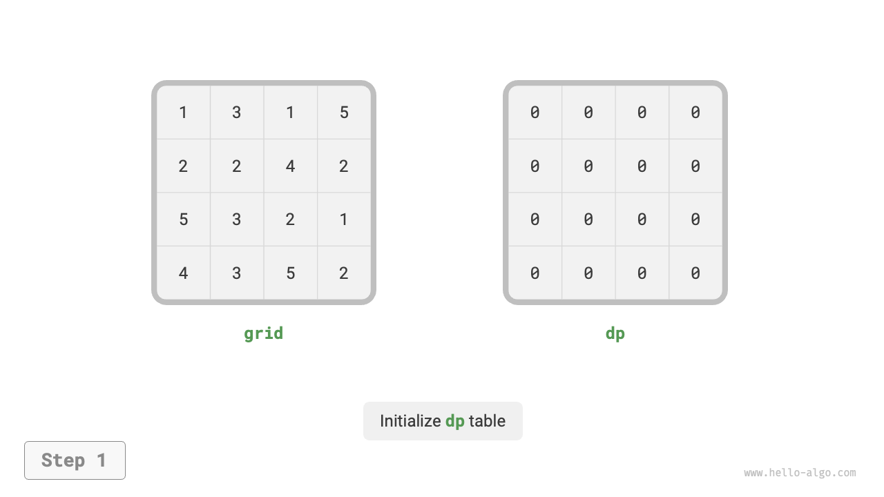


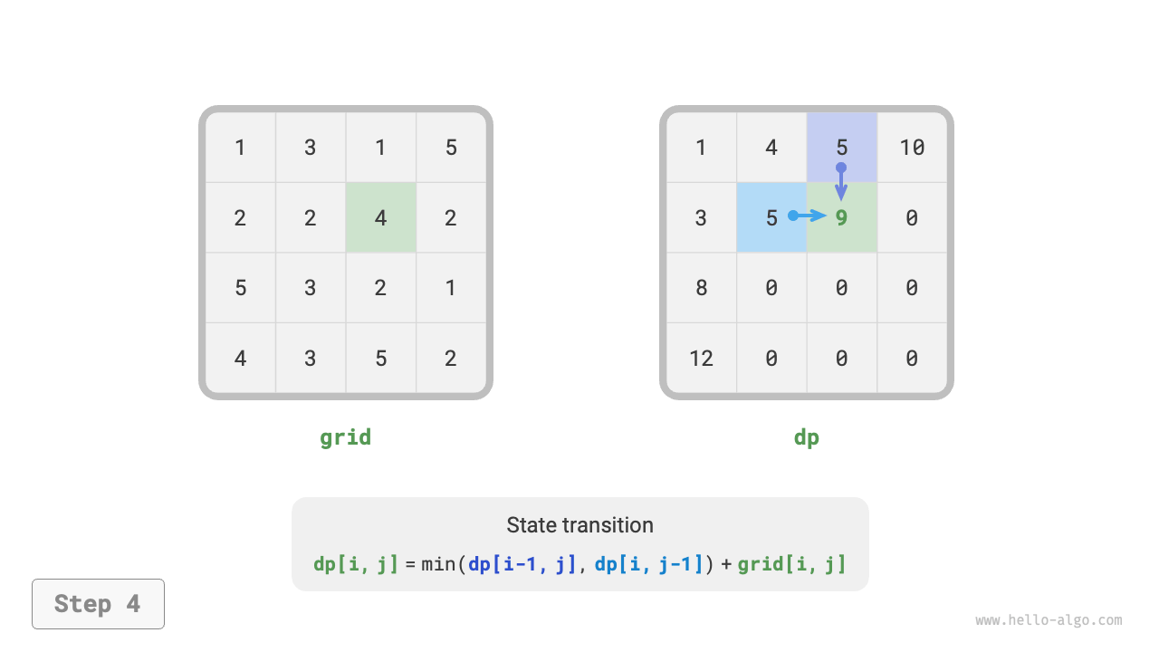


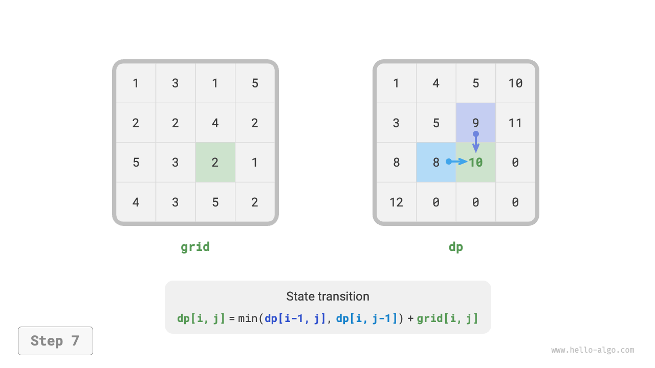


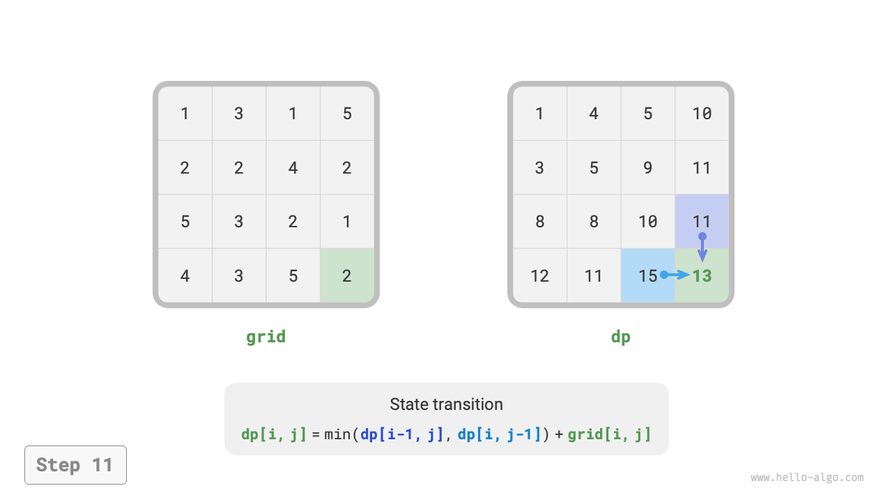
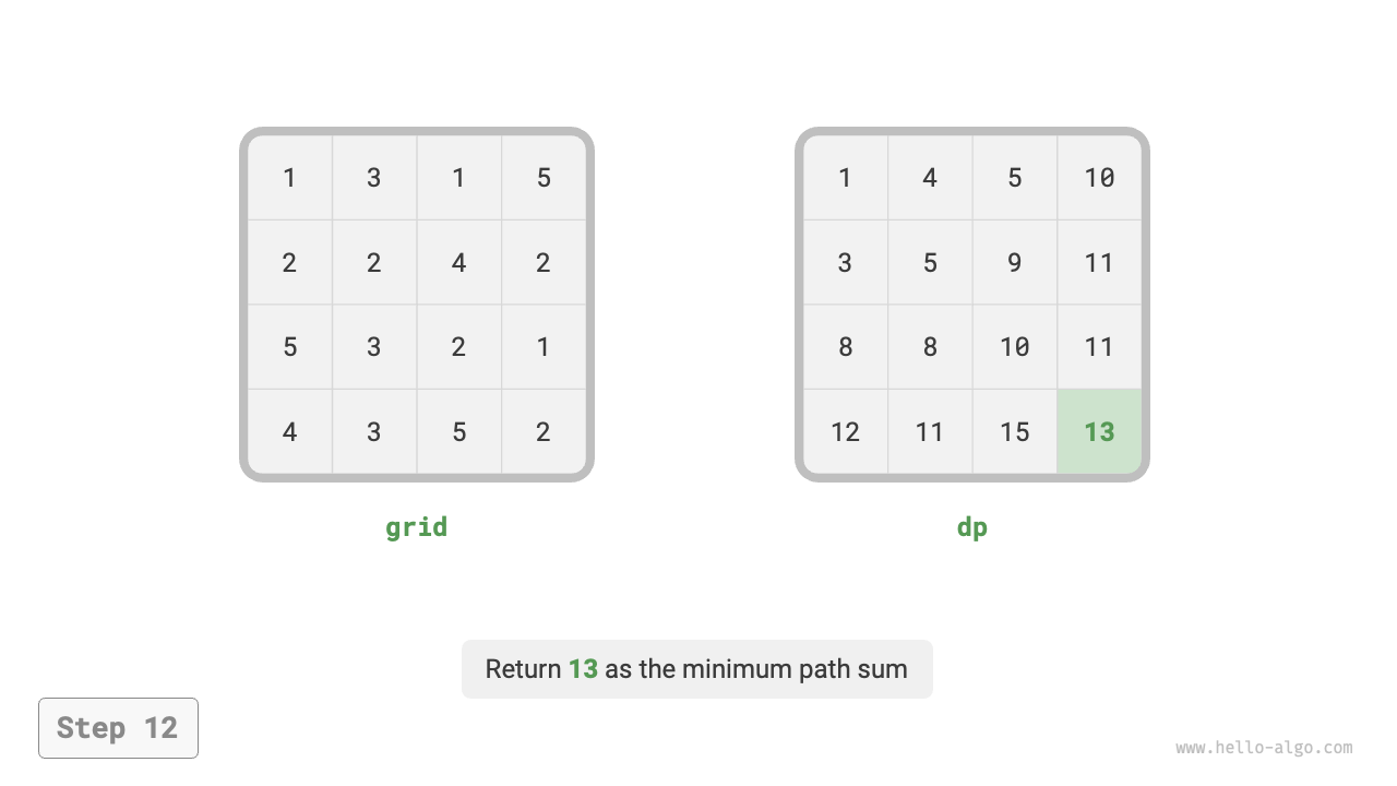
Figure 14-16 Dynamic programming process for minimum path sum
4. Space Optimization
Since each cell is only related to the cell to its left and the cell above it, we can use a single-row array to implement the \(dp\) table.
Note that since the array dp can only represent the state of one row, we cannot initialize the first column state in advance, but rather update it when traversing each row:
def min_path_sum_dp_comp(grid: list[list[int]]) -> int:
    """Minimum path sum: Space-optimized dynamic programming"""
    n, m = len(grid), len(grid[0])
    # Initialize dp table
    dp = [0] * m
    # State transition: first row
    dp[0] = grid[0][0]
    for j in range(1, m):
        dp[j] = dp[j - 1] + grid[0][j]
    # State transition: rest of the rows
    for i in range(1, n):
        # State transition: first column
        dp[0] = dp[0] + grid[i][0]
        # State transition: rest of the columns
        for j in range(1, m):
            dp[j] = min(dp[j - 1], dp[j]) + grid[i][j]
    return dp[m - 1]
/* Minimum path sum: Space-optimized dynamic programming */
int minPathSumDPComp(vector<vector<int>> &grid) {
    int n = grid.size(), m = grid[0].size();
    // Initialize dp table
    vector<int> dp(m);
    // State transition: first row
    dp[0] = grid[0][0];
    for (int j = 1; j < m; j++) {
        dp[j] = dp[j - 1] + grid[0][j];
    }
    // State transition: rest of the rows
    for (int i = 1; i < n; i++) {
        // State transition: first column
        dp[0] = dp[0] + grid[i][0];
        // State transition: rest of the columns
        for (int j = 1; j < m; j++) {
            dp[j] = min(dp[j - 1], dp[j]) + grid[i][j];
        }
    }
    return dp[m - 1];
}
/* Minimum path sum: Space-optimized dynamic programming */
int minPathSumDPComp(int[][] grid) {
    int n = grid.length, m = grid[0].length;
    // Initialize dp table
    int[] dp = new int[m];
    // State transition: first row
    dp[0] = grid[0][0];
    for (int j = 1; j < m; j++) {
        dp[j] = dp[j - 1] + grid[0][j];
    }
    // State transition: rest of the rows
    for (int i = 1; i < n; i++) {
        // State transition: first column
        dp[0] = dp[0] + grid[i][0];
        // State transition: rest of the columns
        for (int j = 1; j < m; j++) {
            dp[j] = Math.min(dp[j - 1], dp[j]) + grid[i][j];
        }
    }
    return dp[m - 1];
}
/* Minimum path sum: Space-optimized dynamic programming */
int MinPathSumDPComp(int[][] grid) {
    int n = grid.Length, m = grid[0].Length;
    // Initialize dp table
    int[] dp = new int[m];
    dp[0] = grid[0][0];
    // State transition: first row
    for (int j = 1; j < m; j++) {
        dp[j] = dp[j - 1] + grid[0][j];
    }
    // State transition: rest of the rows
    for (int i = 1; i < n; i++) {
        // State transition: first column
        dp[0] = dp[0] + grid[i][0];
        // State transition: rest of the columns
        for (int j = 1; j < m; j++) {
            dp[j] = Math.Min(dp[j - 1], dp[j]) + grid[i][j];
        }
    }
    return dp[m - 1];
}
/* Minimum path sum: Space-optimized dynamic programming */
func minPathSumDPComp(grid [][]int) int {
    n, m := len(grid), len(grid[0])
    // Initialize dp table
    dp := make([]int, m)
    // State transition: first row
    dp[0] = grid[0][0]
    for j := 1; j < m; j++ {
        dp[j] = dp[j-1] + grid[0][j]
    }
    // State transition: rest of the rows and columns
    for i := 1; i < n; i++ {
        // State transition: first column
        dp[0] = dp[0] + grid[i][0]
        // State transition: rest of the columns
        for j := 1; j < m; j++ {
            dp[j] = int(math.Min(float64(dp[j-1]), float64(dp[j]))) + grid[i][j]
        }
    }
    return dp[m-1]
}
/* Minimum path sum: Space-optimized dynamic programming */
func minPathSumDPComp(grid: [[Int]]) -> Int {
    let n = grid.count
    let m = grid[0].count
    // Initialize dp table
    var dp = Array(repeating: 0, count: m)
    // State transition: first row
    dp[0] = grid[0][0]
    for j in 1 ..< m {
        dp[j] = dp[j - 1] + grid[0][j]
    }
    // State transition: rest of the rows
    for i in 1 ..< n {
        // State transition: first column
        dp[0] = dp[0] + grid[i][0]
        // State transition: rest of the columns
        for j in 1 ..< m {
            dp[j] = min(dp[j - 1], dp[j]) + grid[i][j]
        }
    }
    return dp[m - 1]
}
/* Minimum path sum: Space-optimized dynamic programming */
function minPathSumDPComp(grid) {
    const n = grid.length,
        m = grid[0].length;
    // Initialize dp table
    const dp = new Array(m);
    // State transition: first row
    dp[0] = grid[0][0];
    for (let j = 1; j < m; j++) {
        dp[j] = dp[j - 1] + grid[0][j];
    }
    // State transition: rest of the rows
    for (let i = 1; i < n; i++) {
        // State transition: first column
        dp[0] = dp[0] + grid[i][0];
        // State transition: rest of the columns
        for (let j = 1; j < m; j++) {
            dp[j] = Math.min(dp[j - 1], dp[j]) + grid[i][j];
        }
    }
    return dp[m - 1];
}
/* Minimum path sum: Space-optimized dynamic programming */
function minPathSumDPComp(grid: Array<Array<number>>): number {
    const n = grid.length,
        m = grid[0].length;
    // Initialize dp table
    const dp = new Array(m);
    // State transition: first row
    dp[0] = grid[0][0];
    for (let j = 1; j < m; j++) {
        dp[j] = dp[j - 1] + grid[0][j];
    }
    // State transition: rest of the rows
    for (let i = 1; i < n; i++) {
        // State transition: first column
        dp[0] = dp[0] + grid[i][0];
        // State transition: rest of the columns
        for (let j = 1; j < m; j++) {
            dp[j] = Math.min(dp[j - 1], dp[j]) + grid[i][j];
        }
    }
    return dp[m - 1];
}
/* Minimum path sum: Space-optimized dynamic programming */
int minPathSumDPComp(List<List<int>> grid) {
  int n = grid.length, m = grid[0].length;
  // Initialize dp table
  List<int> dp = List.filled(m, 0);
  dp[0] = grid[0][0];
  for (int j = 1; j < m; j++) {
    dp[j] = dp[j - 1] + grid[0][j];
  }
  // State transition: rest of the rows
  for (int i = 1; i < n; i++) {
    // State transition: first column
    dp[0] = dp[0] + grid[i][0];
    // State transition: rest of the columns
    for (int j = 1; j < m; j++) {
      dp[j] = min(dp[j - 1], dp[j]) + grid[i][j];
    }
  }
  return dp[m - 1];
}
/* Minimum path sum: Space-optimized dynamic programming */
fn min_path_sum_dp_comp(grid: &Vec<Vec<i32>>) -> i32 {
    let (n, m) = (grid.len(), grid[0].len());
    // Initialize dp table
    let mut dp = vec![0; m];
    // State transition: first row
    dp[0] = grid[0][0];
    for j in 1..m {
        dp[j] = dp[j - 1] + grid[0][j];
    }
    // State transition: rest of the rows
    for i in 1..n {
        // State transition: first column
        dp[0] = dp[0] + grid[i][0];
        // State transition: rest of the columns
        for j in 1..m {
            dp[j] = std::cmp::min(dp[j - 1], dp[j]) + grid[i][j];
        }
    }
    dp[m - 1]
}
/* Minimum path sum: Space-optimized dynamic programming */
int minPathSumDPComp(int grid[MAX_SIZE][MAX_SIZE], int n, int m) {
    // Initialize dp table
    int *dp = calloc(m, sizeof(int));
    // State transition: first row
    dp[0] = grid[0][0];
    for (int j = 1; j < m; j++) {
        dp[j] = dp[j - 1] + grid[0][j];
    }
    // State transition: rest of the rows
    for (int i = 1; i < n; i++) {
        // State transition: first column
        dp[0] = dp[0] + grid[i][0];
        // State transition: rest of the columns
        for (int j = 1; j < m; j++) {
            dp[j] = myMin(dp[j - 1], dp[j]) + grid[i][j];
        }
    }
    int res = dp[m - 1];
    // Free memory
    free(dp);
    return res;
}
/* Minimum path sum: Space-optimized dynamic programming */
fun minPathSumDPComp(grid: Array<IntArray>): Int {
    val n = grid.size
    val m = grid[0].size
    // Initialize dp table
    val dp = IntArray(m)
    // State transition: first row
    dp[0] = grid[0][0]
    for (j in 1..<m) {
        dp[j] = dp[j - 1] + grid[0][j]
    }
    // State transition: rest of the rows
    for (i in 1..<n) {
        // State transition: first column
        dp[0] = dp[0] + grid[i][0]
        // State transition: rest of the columns
        for (j in 1..<m) {
            dp[j] = min(dp[j - 1], dp[j]) + grid[i][j]
        }
    }
    return dp[m - 1]
}
### Minimum path sum: space-optimized DP ###
def min_path_sum_dp_comp(grid)
  n, m = grid.length, grid.first.length
  # Initialize dp table
  dp = Array.new(m, 0)
  # State transition: first row
  dp[0] = grid[0][0]
  (1...m).each { |j| dp[j] = dp[j - 1] + grid[0][j] }
  # State transition: rest of the rows
  for i in 1...n
    # State transition: first column
    dp[0] = dp[0] + grid[i][0]
    # State transition: rest of the columns
    (1...m).each { |j| dp[j] = [dp[j - 1], dp[j]].min + grid[i][j] }
  end
  dp[m - 1]
end