15.1 Greedy Algorithm
Greedy algorithm is a common approach to solving optimization problems. Its basic idea is to choose the option that appears best at each decision stage, that is, to greedily make locally optimal decisions in the hope of obtaining a globally optimal solution. Greedy algorithms are simple and efficient, and are widely used in many practical problems.
Greedy algorithms and dynamic programming are both commonly used to solve optimization problems. They share some similarities, such as both relying on the optimal substructure property, but they work differently.
- Dynamic programming considers all previous decisions when making the current decision, and uses solutions to past subproblems to construct the solution to the current subproblem.
- Greedy algorithms do not consider past decisions, but instead make greedy choices moving forward, continually reducing the problem size until the problem is solved.
We will first understand how greedy algorithms work through the example problem "coin change." This problem was already introduced in the "Complete Knapsack Problem" chapter, so it should already be familiar to you.
Question
Given \(n\) types of coins, where the denomination of the \(i\)-th type is \(coins[i - 1]\), a target amount \(amt\), and an unlimited number of coins of each type, what is the minimum number of coins needed to make up the target amount? If the target amount cannot be made up, return \(-1\).
The greedy strategy for this problem is shown in Figure 15-1. Given a target amount, we greedily choose the coin that does not exceed it and is closest to it, repeating this step until the target amount is made up.
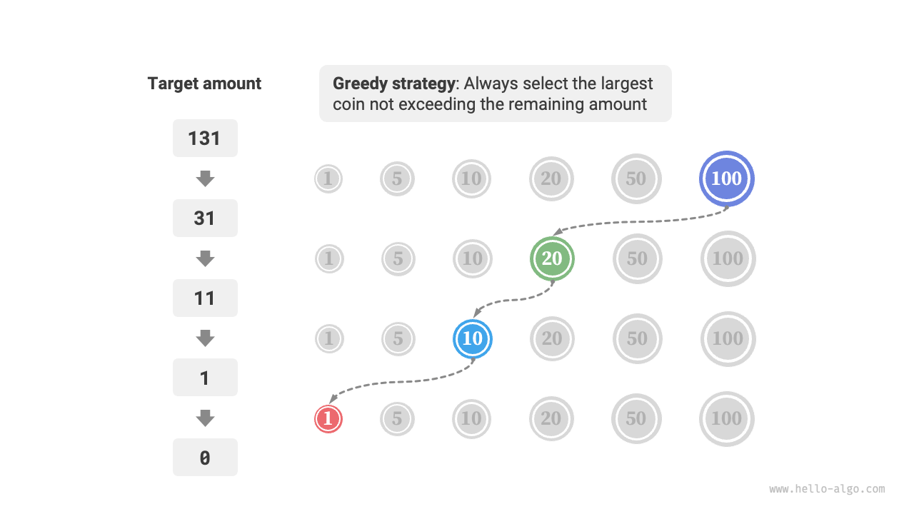
Figure 15-1 Greedy strategy for coin change
The implementation code is as follows:
def coin_change_greedy(coins: list[int], amt: int) -> int:
    """Coin change: Greedy algorithm"""
    # Assume coins list is sorted
    i = len(coins) - 1
    count = 0
    # Loop to make greedy choices until no remaining amount
    while amt > 0:
        # Find the coin that is less than and closest to the remaining amount
        while i > 0 and coins[i] > amt:
            i -= 1
        # Choose coins[i]
        amt -= coins[i]
        count += 1
    # If no feasible solution is found, return -1
    return count if amt == 0 else -1
/* Coin change: Greedy algorithm */
int coinChangeGreedy(vector<int> &coins, int amt) {
    // Assume coins list is sorted
    int i = coins.size() - 1;
    int count = 0;
    // Loop to make greedy choices until no remaining amount
    while (amt > 0) {
        // Find the coin that is less than and closest to the remaining amount
        while (i > 0 && coins[i] > amt) {
            i--;
        }
        // Choose coins[i]
        amt -= coins[i];
        count++;
    }
    // If no feasible solution is found, return -1
    return amt == 0 ? count : -1;
}
/* Coin change: Greedy algorithm */
int coinChangeGreedy(int[] coins, int amt) {
    // Assume coins list is sorted
    int i = coins.length - 1;
    int count = 0;
    // Loop to make greedy choices until no remaining amount
    while (amt > 0) {
        // Find the coin that is less than and closest to the remaining amount
        while (i > 0 && coins[i] > amt) {
            i--;
        }
        // Choose coins[i]
        amt -= coins[i];
        count++;
    }
    // If no feasible solution is found, return -1
    return amt == 0 ? count : -1;
}
/* Coin change: Greedy algorithm */
int CoinChangeGreedy(int[] coins, int amt) {
    // Assume coins list is sorted
    int i = coins.Length - 1;
    int count = 0;
    // Loop to make greedy choices until no remaining amount
    while (amt > 0) {
        // Find the coin that is less than and closest to the remaining amount
        while (i > 0 && coins[i] > amt) {
            i--;
        }
        // Choose coins[i]
        amt -= coins[i];
        count++;
    }
    // If no feasible solution is found, return -1
    return amt == 0 ? count : -1;
}
/* Coin change: Greedy algorithm */
func coinChangeGreedy(coins []int, amt int) int {
    // Assume coins list is sorted
    i := len(coins) - 1
    count := 0
    // Loop to make greedy choices until no remaining amount
    for amt > 0 {
        // Find the coin that is less than and closest to the remaining amount
        for i > 0 && coins[i] > amt {
            i--
        }
        // Choose coins[i]
        amt -= coins[i]
        count++
    }
    // If no feasible solution is found, return -1
    if amt != 0 {
        return -1
    }
    return count
}
/* Coin change: Greedy algorithm */
func coinChangeGreedy(coins: [Int], amt: Int) -> Int {
    // Assume coins list is sorted
    var i = coins.count - 1
    var count = 0
    var amt = amt
    // Loop to make greedy choices until no remaining amount
    while amt > 0 {
        // Find the coin that is less than and closest to the remaining amount
        while i > 0 && coins[i] > amt {
            i -= 1
        }
        // Choose coins[i]
        amt -= coins[i]
        count += 1
    }
    // If no feasible solution is found, return -1
    return amt == 0 ? count : -1
}
/* Coin change: Greedy algorithm */
function coinChangeGreedy(coins, amt) {
    // Assume coins array is sorted
    let i = coins.length - 1;
    let count = 0;
    // Loop to make greedy choices until no remaining amount
    while (amt > 0) {
        // Find the coin that is less than and closest to the remaining amount
        while (i > 0 && coins[i] > amt) {
            i--;
        }
        // Choose coins[i]
        amt -= coins[i];
        count++;
    }
    // If no feasible solution is found, return -1
    return amt === 0 ? count : -1;
}
/* Coin change: Greedy algorithm */
function coinChangeGreedy(coins: number[], amt: number): number {
    // Assume coins array is sorted
    let i = coins.length - 1;
    let count = 0;
    // Loop to make greedy choices until no remaining amount
    while (amt > 0) {
        // Find the coin that is less than and closest to the remaining amount
        while (i > 0 && coins[i] > amt) {
            i--;
        }
        // Choose coins[i]
        amt -= coins[i];
        count++;
    }
    // If no feasible solution is found, return -1
    return amt === 0 ? count : -1;
}
/* Coin change: Greedy algorithm */
int coinChangeGreedy(List<int> coins, int amt) {
  // Assume coins list is sorted
  int i = coins.length - 1;
  int count = 0;
  // Loop to make greedy choices until no remaining amount
  while (amt > 0) {
    // Find the coin that is less than and closest to the remaining amount
    while (i > 0 && coins[i] > amt) {
      i--;
    }
    // Choose coins[i]
    amt -= coins[i];
    count++;
  }
  // If no feasible solution is found, return -1
  return amt == 0 ? count : -1;
}
/* Coin change: Greedy algorithm */
fn coin_change_greedy(coins: &[i32], mut amt: i32) -> i32 {
    // Assume coins list is sorted
    let mut i = coins.len() - 1;
    let mut count = 0;
    // Loop to make greedy choices until no remaining amount
    while amt > 0 {
        // Find the coin that is less than and closest to the remaining amount
        while i > 0 && coins[i] > amt {
            i -= 1;
        }
        // Choose coins[i]
        amt -= coins[i];
        count += 1;
    }
    // If no feasible solution is found, return -1
    if amt == 0 {
        count
    } else {
        -1
    }
}
/* Coin change: Greedy algorithm */
int coinChangeGreedy(int *coins, int size, int amt) {
    // Assume coins list is sorted
    int i = size - 1;
    int count = 0;
    // Loop to make greedy choices until no remaining amount
    while (amt > 0) {
        // Find the coin that is less than and closest to the remaining amount
        while (i > 0 && coins[i] > amt) {
            i--;
        }
        // Choose coins[i]
        amt -= coins[i];
        count++;
    }
    // If no feasible solution is found, return -1
    return amt == 0 ? count : -1;
}
/* Coin change: Greedy algorithm */
fun coinChangeGreedy(coins: IntArray, amt: Int): Int {
    // Assume coins list is sorted
    var am = amt
    var i = coins.size - 1
    var count = 0
    // Loop to make greedy choices until no remaining amount
    while (am > 0) {
        // Find the coin that is less than and closest to the remaining amount
        while (i > 0 && coins[i] > am) {
            i--
        }
        // Choose coins[i]
        am -= coins[i]
        count++
    }
    // If no feasible solution is found, return -1
    return if (am == 0) count else -1
}
### Coin change: greedy ###
def coin_change_greedy(coins, amt)
  # Assume coins list is sorted
  i = coins.length - 1
  count = 0
  # Loop to make greedy choices until no remaining amount
  while amt > 0
    # Find the coin that is less than and closest to the remaining amount
    while i > 0 && coins[i] > amt
      i -= 1
    end
    # Choose coins[i]
    amt -= coins[i]
    count += 1
  end
  # Return -1 if no solution found
  amt == 0 ? count : -1
end
You may find yourself exclaiming, "So clean!" The greedy algorithm solves the coin change problem in only about ten lines of code.
15.1.1 Advantages and Limitations of Greedy Algorithms
Greedy algorithms are not only straightforward to apply and easy to implement, but are also usually very efficient. In the code above, if the smallest coin denomination is \(\min(coins)\), the greedy selection loop runs at most \(amt / \min(coins)\) times, giving a time complexity of \(O(amt / \min(coins))\). This is an order of magnitude lower than the time complexity of the dynamic programming solution, \(O(n \times amt)\).
However, for some coin denomination sets, greedy algorithms cannot find the optimal solution. Figure 15-2 shows two examples.
- Positive example \(coins = [1, 5, 10, 20, 50, 100]\): With this coin set, the greedy algorithm can find the optimal solution for any \(amt\).
- Counterexample \(coins = [1, 20, 50]\): Suppose \(amt = 60\). The greedy algorithm can only find the combination \(50 + 1 \times 10\), using \(11\) coins in total, whereas dynamic programming can find the optimal solution \(20 + 20 + 20\) using only \(3\) coins.
- Counterexample \(coins = [1, 49, 50]\): Suppose \(amt = 98\). The greedy algorithm can only find the combination \(50 + 1 \times 48\), using \(49\) coins in total, whereas dynamic programming can find the optimal solution \(49 + 49\) using only \(2\) coins.
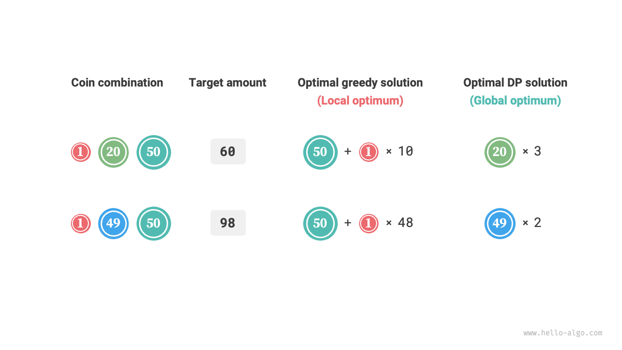
Figure 15-2 Examples where greedy algorithms cannot find the optimal solution
In other words, for the coin change problem, greedy algorithms cannot guarantee a globally optimal solution and may even produce very poor results. This problem is better solved with dynamic programming.
In general, greedy algorithms are applicable in the following two situations.
- The optimal solution can be guaranteed: In this case, greedy algorithms are often the best choice because they tend to be more efficient than backtracking and dynamic programming.
- An approximately optimal solution can be found: Greedy algorithms are also useful in this case. For many complex problems, finding the global optimal solution is very difficult, so efficiently finding a suboptimal solution is already a very good outcome.
15.1.2 Characteristics of Greedy Algorithms
So the question arises: what kind of problems are suitable for solving with greedy algorithms? Or in other words, under what conditions can greedy algorithms guarantee finding the optimal solution?
Compared to dynamic programming, the conditions for using greedy algorithms are stricter, mainly focusing on two properties of the problem.
- Greedy choice property: Only when locally optimal choices can always lead to a globally optimal solution can greedy algorithms guarantee obtaining the optimal solution.
- Optimal substructure: The optimal solution to the original problem contains the optimal solutions to subproblems.
Optimal substructure has already been introduced in the "Dynamic Programming" chapter, so we won't elaborate on it here. It's worth noting that the optimal substructure of some problems is not obvious, but they can still be solved using greedy algorithms.
We mainly explore methods for determining the greedy choice property. Although its description seems relatively simple, in practice, for many problems, proving the greedy choice property is not easy.
For example, in the coin change problem, although we can easily provide counterexamples to disprove the greedy choice property, proving that it holds is much harder. If asked, under what conditions can a coin set be solved using a greedy algorithm? We often can only rely on intuition or examples to give a vague answer, and it is difficult to provide a rigorous mathematical proof.
Quote
There is a paper that presents an \(O(n^3)\) algorithm for determining whether a coin set can be solved optimally by a greedy algorithm for any amount.
Pearson, D. A polynomial-time algorithm for the change-making problem[J]. Operations Research Letters, 2005, 33(3): 231-234.
15.1.3 Steps for Solving Problems with Greedy Algorithms
The general process for solving greedy problems can be divided into the following three steps.
- Problem analysis: Sort out and understand the characteristics of the problem, including state definitions, optimization objectives, and constraints. This step also appears in backtracking and dynamic programming.
- Determine the greedy strategy: Decide how to make a greedy choice at each step. This strategy should reduce the problem size step by step and ultimately solve the entire problem.
- Correctness proof: It is usually necessary to prove that the problem has both greedy choice property and optimal substructure. This step may require mathematical tools such as induction or proof by contradiction.
Determining the greedy strategy is the core step in solving such problems, but it may not be easy in practice, mainly for the following reasons.
- Greedy strategies vary greatly from problem to problem. For many problems, the greedy strategy is fairly intuitive and can be derived through rough reasoning and experimentation. For some complex problems, however, the greedy strategy may be deeply hidden, which strongly tests one's problem-solving experience and algorithmic ability.
- Some greedy strategies are highly deceptive. We may confidently design a greedy strategy, write the solution code, and submit it, only to find that some test cases fail. This is because the designed greedy strategy is only "partially correct," as exemplified by the coin change problem discussed above.
To ensure correctness, we should give a rigorous mathematical proof of the greedy strategy, usually using proof by contradiction or mathematical induction.
However, correctness proofs can also be difficult. If we have no clear direction, we usually resort to debugging against test cases, revising and validating the greedy strategy step by step.
15.1.4 Typical Problems Solved by Greedy Algorithms
Greedy algorithms are often applied to optimization problems that satisfy greedy choice property and optimal substructure. Below are some typical greedy algorithm problems.
- Coin change problem: With certain coin combinations, greedy algorithms can always obtain the optimal solution.
- Interval scheduling problem: Suppose you have some tasks, each taking place during a period of time, and your goal is to complete as many tasks as possible. If you always choose the task that ends earliest, then the greedy algorithm can obtain the optimal solution.
- Fractional knapsack problem: Given a set of items and a carrying capacity, your goal is to select a set of items such that the total weight does not exceed the carrying capacity and the total value is maximized. If you always choose the item with the highest value-to-weight ratio (value / weight), then the greedy algorithm can obtain the optimal solution in some cases.
- Stock trading problem: Given a set of historical stock prices, you can make multiple trades, but if you already hold stocks, you cannot buy again before selling, and the goal is to obtain the maximum profit.
- Huffman coding: Huffman coding is a greedy algorithm used for lossless data compression. By constructing a Huffman tree and always merging the two nodes with the lowest frequency, the resulting Huffman tree has the minimum weighted path length (encoding length).
- Dijkstra's algorithm: It is a greedy algorithm for solving the shortest path problem from a given source vertex to all other vertices.